Superstore Global Sales Analysis
- Dataset
- Data loading
- Data cleansing
- Preparation for analysis
- Analysis
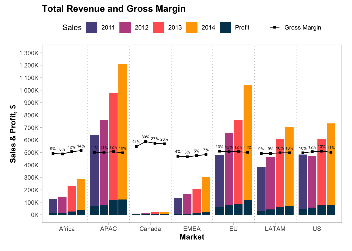
- Total Revenue and Gross Margin
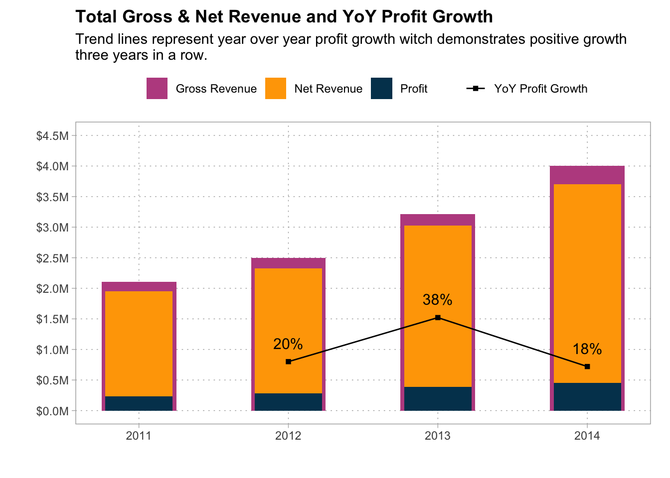
- Total Gross & Net Revenue and YoY Profit Growth
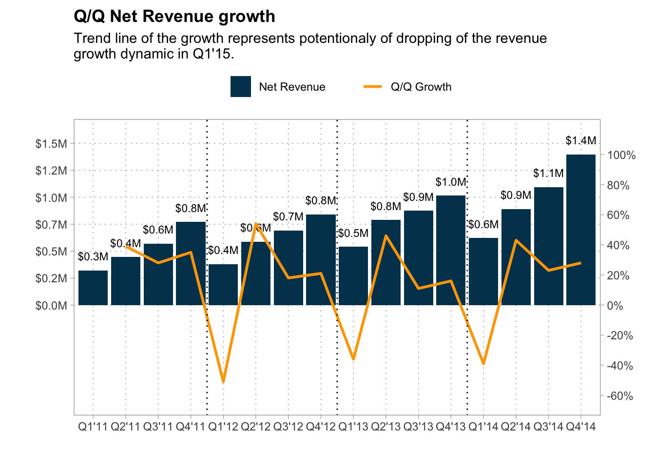
- Quarterly Net Revenue growth
- Profit trends
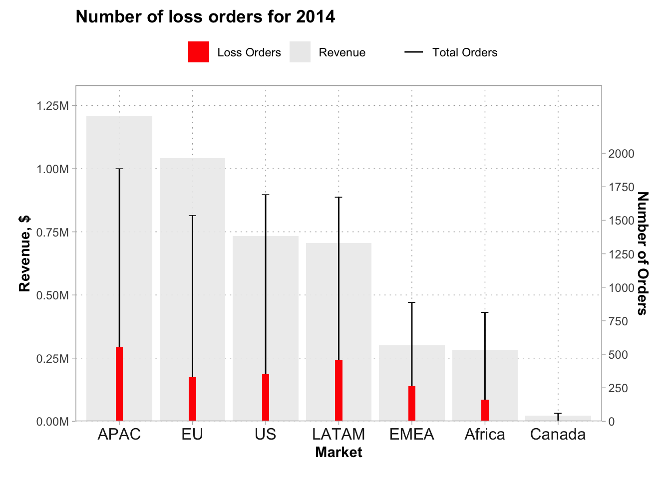
- Total number of orders and loss orders
- Customer Lifetime Value (CLV)
- Quarterly Customer Retention Rate
- ARPPU and Average check value
- Average Basket Value and size
- Return Rate
- What most significant sub-categories?
- Map
- Top 10 countries by Sales Volume
- Sales analysis heat map by day and month
- Top 5 returnable sub-categories by merket
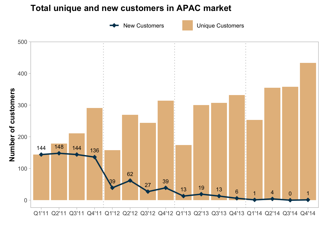
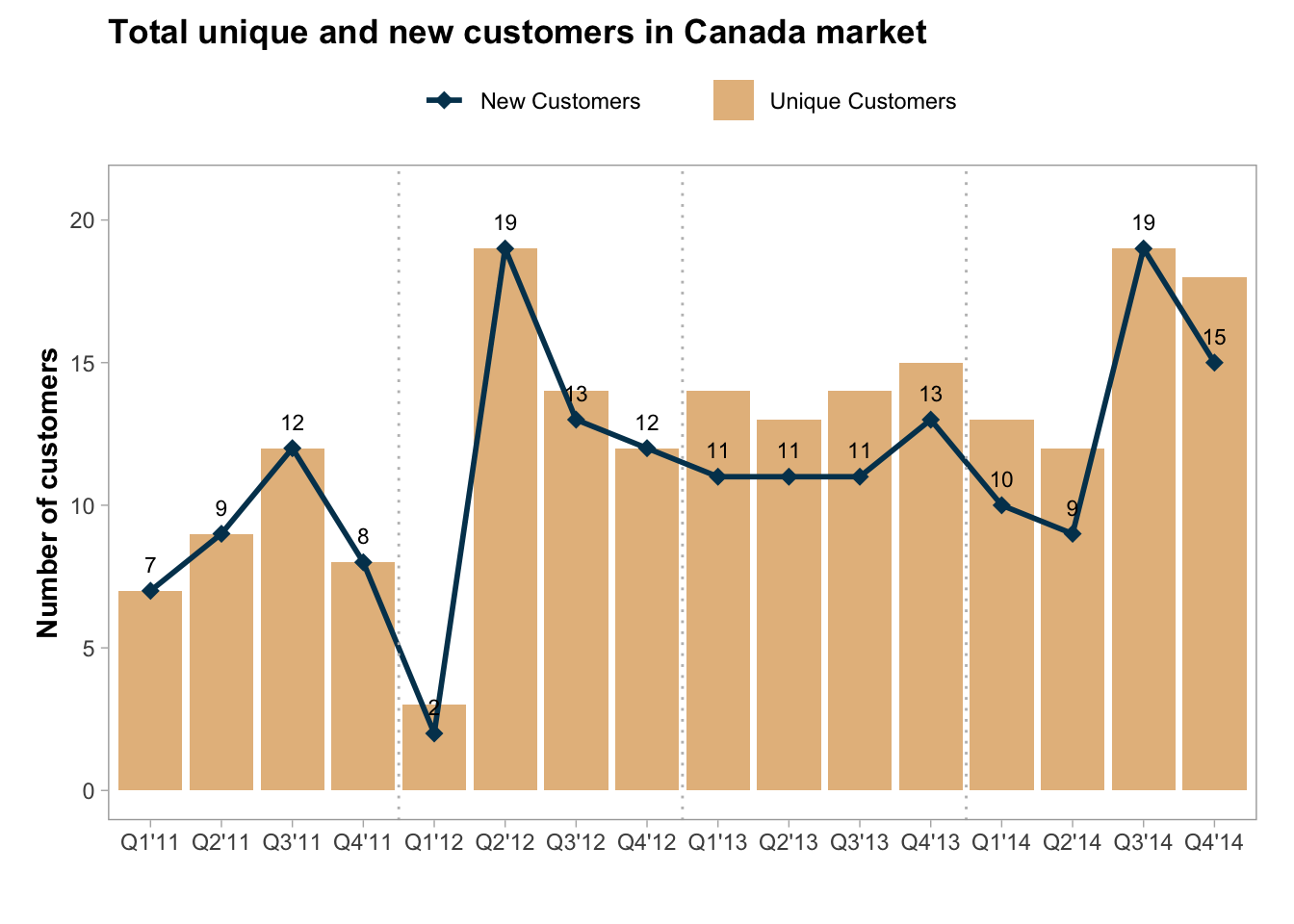
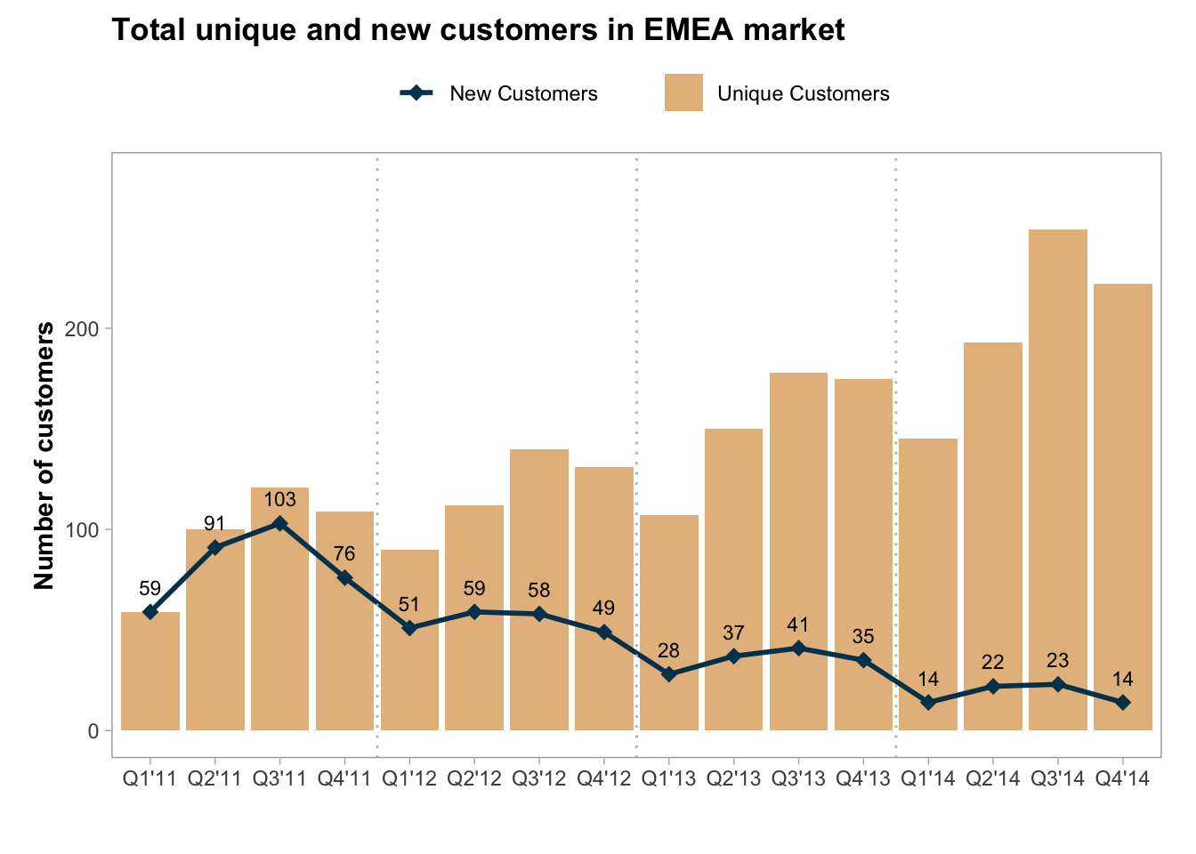
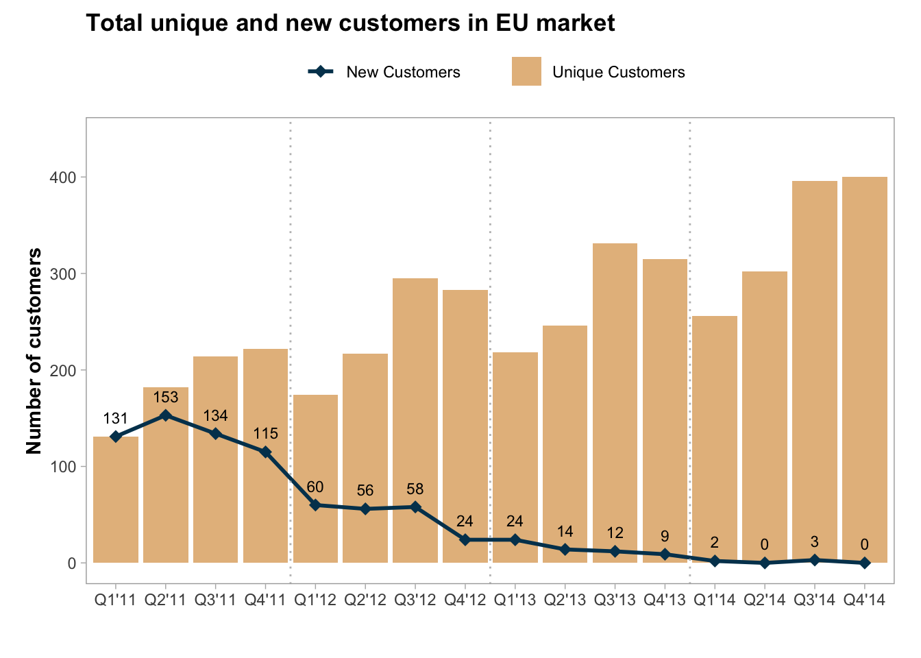
- What are number of total and new customers?
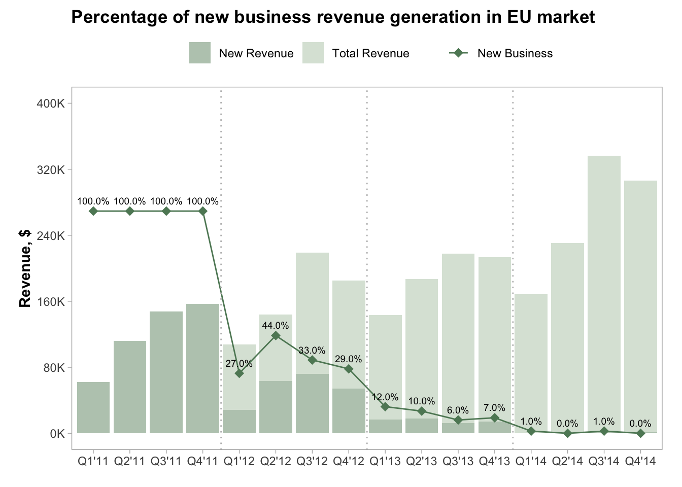
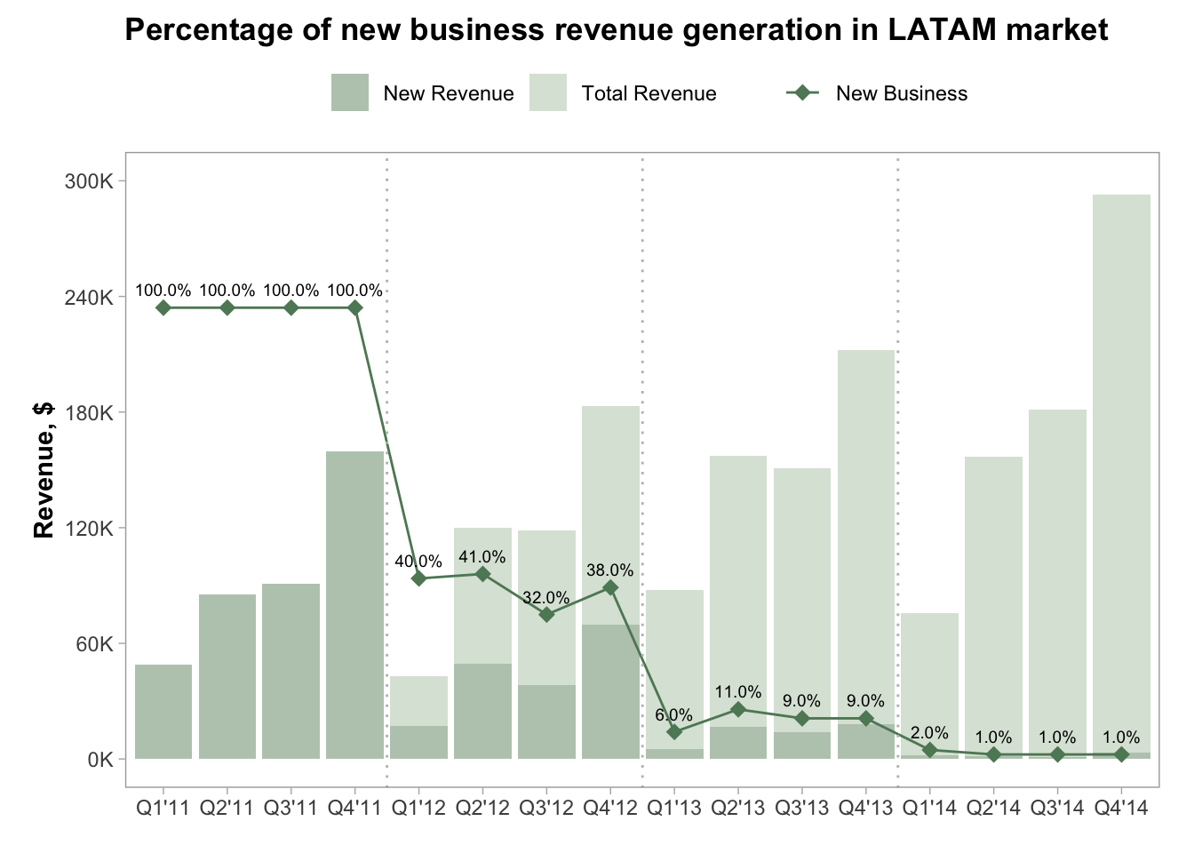
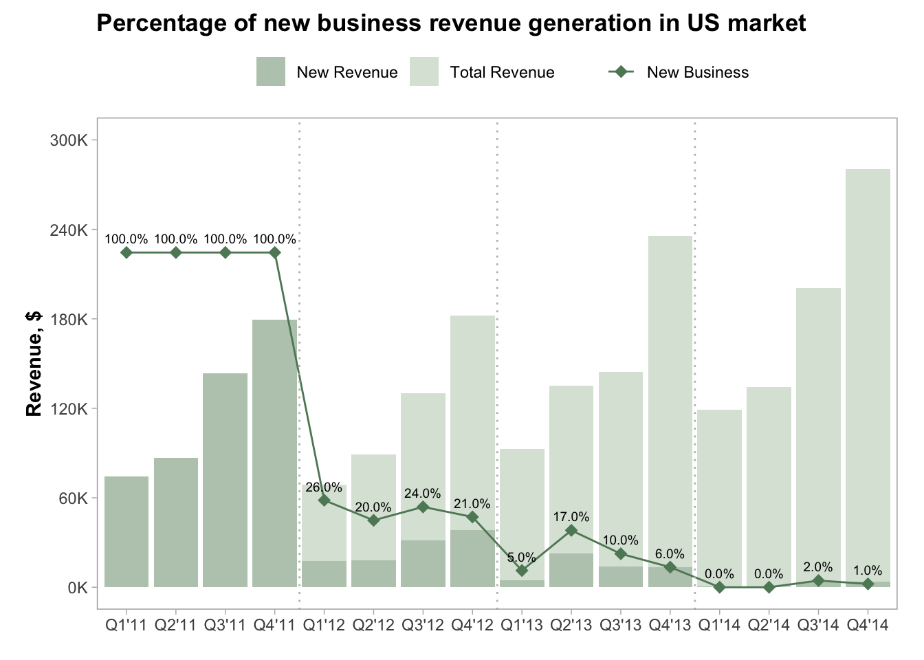
- Percentage of new business revenue generation
# loading libraries
library(DBI)
library(RPostgres)
library(ggplot2)
library(forcats)
library(stringi)
library(kableExtra)
library(RColorBrewer)
library(treemapify)
library(knitr)
library(tidyverse)
library(tidygeocoder)
library(formatR)
Dataset
The Global Superstore dataset contains data of transactions, each row represents transaction item of products sold around the world by Superstore, also contains a customer information, shipping and product returns.
Metadata
The dataset contains the following tables:
Table Orders
| Variable name | Data type | Description |
|---|---|---|
| Row ID | Integer |
Unique ID for each row. |
| Order ID | String |
Unique Order ID for each Customer. |
| Order Date | Date |
Order Date of the product. |
| Ship Date | Date |
Shipping Date of the Product. |
| Ship Mode | String |
Shipping Mode specified by the Customer. |
| Customer ID | String |
Unique ID to identify each Customer. |
| Customer Name | String |
Name of the Customer. |
| Segment | String |
The segment where the Customer belongs. |
| City | String |
City of residence of of the Customer. |
| State | String |
State of residence of the Customer. |
| Country | String |
Country of residence of the Customer. |
| Postal Code | String |
Postal Code of residence of the Customer. |
| Market | String |
Market name. |
| Region | String |
Region where the Customer belong. |
| Product ID | String |
Unique ID of the Product. |
| Category | String |
Category of the product ordered. |
| Sub-Category | String |
Sub-Category of the product ordered. |
| Product Name | String |
Name of the Product |
| Sales | Decimal |
Sales of the Product. |
| Quantity | Integer |
Quantity of the Product. |
| Discount | Decimal |
Discount provided. |
| Profit | Decimal |
Profit/Loss incurred. |
| Shipping Cost | Decimal |
Shipping cost. |
| Order Priority | String |
Order priority. |
Table Returns
| Variable name | Data type | Description |
|---|---|---|
| Order ID | String |
Unique Order ID for each Customer. |
| Returned | Bool |
The flag, indicates that the order was returned. |
| Market | String |
Market name. |
Data loading
# DB connection
con <- dbConnect(
  RPostgres::Postgres(), dbname = "superstore_global",
  host = "localhost", port = 5432, user = "postgres",
  password = ""
)
For analysis for used PostgreSQL database.
-- NOTE: you need to execute the code below on DB side (R Markdown chunk eval=FALSE).

-- Create a new database
CREATE DATABASE superstore_global;
-- create table Orders for raw data
CREATE TABLE raw_data.superstore_orders
(
row_id VARCHAR(5),
order_id VARCHAR(15),
order_date VARCHAR(10),
ship_date VARCHAR(10),
ship_mode VARCHAR(14),
customer_id VARCHAR(8),
customer_name VARCHAR(22),
segment VARCHAR(11),
city VARCHAR(35),
state VARCHAR(36),
country VARCHAR(32),
postal_code VARCHAR(5),
market VARCHAR(6),
region VARCHAR(14),
product_id VARCHAR(16),
category VARCHAR(15),
sub_category VARCHAR(11),
product_name VARCHAR(127),
sales VARCHAR(10),
quantity VARCHAR(2),
discount VARCHAR(5),
profit VARCHAR(21),
shipping_cost VARCHAR(8),
order_priority VARCHAR(8)
);-- NOTE: you need to execute the code below on DB side (R Markdown chunk eval=FALSE).
-- create table Returns for raw data
CREATE TABLE raw_data.superstore_returns
(
returned VARCHAR(3),
order_id VARCHAR(15),
market VARCHAR(13)
);Prepare data in Excel. Save each sheet as CSV file: + Sheet Orders into data/Global Superstore_orders.csv. + Sheet Returns into data/Global Superstore_returns.csv.
library(readxl)
library(fs)

file_name <- "Global Superstore (raw data).xls"
sheets <- readxl::excel_sheets(paste0("./data/", file_name))
CSVs <- c()
for (sheet in sheets[1:2]) {
  df <- readxl::read_xls(
    paste0("./data/", file_name),
    col_names = TRUE, sheet = sheet
  )
  csv_file <- paste0(
    getwd(), "/data/", "Global Superstore_", sheet,
    ".csv"
  )
  CSVs <- append(CSVs, csv_file)
  write.csv(df, csv_file, row.names = FALSE)
}

orders_csv <- CSVs[1]
returns_csv <- CSVs[2]
Now load data as-is into database. Loading raw data.
Data cleansing
Create schema analysis for cleaned data.
Create tables for cleaned data.
CREATE TABLE analysis.orders
(
    row_id         INTEGER,
    order_id       VARCHAR(15),
    order_date     DATE,
    ship_date      DATE,
    ship_mode      VARCHAR(14),
    customer_id    VARCHAR(8),
    customer_name  VARCHAR(22),
    segment        VARCHAR(11),
    city           VARCHAR(35),
    state          VARCHAR(36),
    country        VARCHAR(32),
    postal_code    VARCHAR(5),
    market         VARCHAR(6),
    region         VARCHAR(14),
    product_id     VARCHAR(16),
    category       VARCHAR(15),
    sub_category   VARCHAR(11),
    product_name   VARCHAR(127),
    sales          NUMERIC(9, 2),
    quantity       SMALLINT,
    discount       NUMERIC(4, 2),
    profit         NUMERIC(9, 2),
    shipping_cost  NUMERIC(9, 2),
    order_priority VARCHAR(8)
);Convert data types.
-- Orders table
INSERT INTO analysis.orders
SELECT CAST(row_id AS INTEGER)                                 AS row_id,
       order_id,
       TO_DATE(order_date, 'YYYY-MM-DD')                       AS order_date,
       TO_DATE(ship_date, 'YYYY-MM-DD')                        AS ship_date,
       ship_mode,
       customer_id,
       customer_name,
       segment,
       city,
       state,
       country,
       postal_code,
       market,
       region,
       product_id,
       category,
       sub_category,
       product_name,
       CAST(REPLACE(sales, ',', '.') AS NUMERIC(9, 2))         AS sales,
       CAST(quantity AS SMALLINT)                              AS quantity,
       CAST(REPLACE(discount, ',', '.') AS NUMERIC(4, 2))      AS discount,
       CAST(REPLACE(profit, ',', '.') AS NUMERIC(9, 2))        AS profit,
       CAST(REPLACE(shipping_cost, ',', '.') AS NUMERIC(9, 2)) AS shipping_cost,
       order_priority
FROM raw_data.superstore_orders;
-- Returns table
INSERT INTO analysis.returns
SELECT CAST(returned AS BOOLEAN) AS returned,
order_id,
market
FROM raw_data.superstore_returns;Check Returns table.
SELECT orders.market, returns.market
FROM
(SELECT DISTINCT market FROM analysis.orders ORDER BY 1) AS orders
FULL JOIN
(SELECT DISTINCT market FROM analysis.returns ORDER BY 1) AS returns
ON orders.market = returns.market;Fix market name in Returns table.
Duplication Data
Check duplicated pairs of order_id and market in returns table.
-- duplicated data
SELECT
    row_id,
    order_id,
    order_date,
    ship_date,
    ship_mode,
    customer_id,
    customer_name,
    segment,
    city,
    state,
    country,
    postal_code,
    market,
    region,
    product_id,
    category,
    sub_category,
    product_name,
    sales,
    quantity,
    discount,
    profit,
    shipping_cost,
    order_priority, count(*)
FROM analysis.orders
GROUP BY 1,2,3,4,5,6,7,8,9,10,11,12,13,14,15,16,17,18,19,20,21,22,23,24
having count(*) > 1;Check duplicates without row_id.
SELECT
    order_id,
    order_date,
    ship_date,
    ship_mode,
    customer_id,
    customer_name,
    segment,
    city,
    state,
    country,
    postal_code,
    market,
    region,
    product_id,
    category,
    sub_category,
    product_name,
    sales,
    quantity,
    discount,
    profit,
    shipping_cost,
    order_priority, count(*)
FROM analysis.orders
GROUP BY 1,2,3,4,5,6,7,8,9,10,11,12,13,14,15,16,17,18,19,20,21,22,23
having count(*) > 1;Missing Values
select count(1) FILTER ( WHERE row_id is NULL ) AS row_id,
       count(1) FILTER ( WHERE order_id IS NULL ) AS order_id,
       count(1) FILTER ( WHERE order_date IS NULL ) AS order_date,
       count(1) FILTER ( WHERE ship_date IS NULL ) AS ship_date,
       count(1) FILTER ( WHERE ship_mode IS NULL ) AS ship_mode,
       count(1) FILTER ( WHERE customer_id IS NULL ) AS customer_id,
       count(1) FILTER ( WHERE customer_name IS NULL ) AS customer_name,
       count(1) FILTER ( WHERE segment IS NULL ) AS segment,
       count(1) FILTER ( WHERE city IS NULL ) AS city,
       count(1) FILTER ( WHERE state IS NULL ) AS state,
       count(1) FILTER ( WHERE country IS NULL ) AS country,
       count(1) FILTER ( WHERE postal_code IS NULL ) AS postal_code,
       count(1) FILTER ( WHERE market IS NULL ) AS market,
       count(1) FILTER ( WHERE region IS NULL ) AS region,
       count(1) FILTER ( WHERE product_id IS NULL ) AS product_id,
       count(1) FILTER ( WHERE category IS NULL ) AS category,
       count(1) FILTER ( WHERE sub_category IS NULL ) AS sub_category,
       count(1) FILTER ( WHERE product_name IS NULL ) AS product_name,
       count(1) FILTER ( WHERE sales IS NULL ) AS sales,
       count(1) FILTER ( WHERE quantity IS NULL ) AS quantity,
       count(1) FILTER ( WHERE discount IS NULL ) AS discount,
       count(1) FILTER ( WHERE profit IS NULL ) AS profit,
       count(1) FILTER ( WHERE shipping_cost IS NULL ) AS shipping_cost,
       count(1) FILTER ( WHERE order_priority IS NULL ) AS order_priority
FROM analysis.orders;Preparation for analysis
Make materialized view.
Analysis
# setup plots theme
theme_set(theme_light())
theme_update(
  axis.title = element_text(face = "bold"),
  plot.title = element_text(face = "bold"),
  panel.grid.major = element_line(color = "darkgray", linetype = "dotted"),
  panel.grid.minor = element_blank(), panel.background = element_blank(),
  panel.border = element_rect(color = "darkgray"),
  plot.margin = unit(
    c(0.5, 1, 1, 1),
    "lines"
  )
)
Total Revenue and Gross Margin
SELECT DATE_PART('year', order_date)::INT                     AS year,
       market,
       round(SUM(sales), 2)                                   AS sales,
       round(SUM(profit) FILTER (WHERE NOT returned), 2)      AS profit, -- exclude returns
       round(SUM(profit) FILTER (WHERE NOT returned) / SUM(sales), 2) AS margin
FROM analysis.all_global_orders
GROUP BY 1, 2
ORDER BY year, sales desc;
scale <- mean(revenue_margin$sales)
offset <- mean(revenue_margin$sales)

ggplot(revenue_margin) +
  geom_bar(
    aes(x = market, y = sales, fill = factor(year)),
    stat = "identity", position = position_dodge2(width = 0.9)
  ) +
  geom_bar(
    aes(x = market, y = profit, fill = "Profit"),
    stat = "identity", position = position_dodge2(width = 0.9)
  ) +
  geom_line(
    aes(
      x = market, y = offset + margin * scale,
      group = market, color = "Gross Margin"
    ),
    position = position_dodge2(width = 0.9)
  ) +
  geom_point(
    aes(
      x = market, y = offset + margin * scale,
      color = "Gross Margin"
    ),
    position = position_dodge2(width = 0.9),
    shape = 15
  ) +
  geom_text(
    aes(
      x = market, y = offset + margin * scale,
      label = scales::percent(margin, accuracy = 1L)
    ),
    vjust = -1.2, position = position_dodge2(width = 0.9),
    size = 2
  ) +
  geom_vline(
    xintercept = seq(
      1.5, length(unique(revenue_margin$market)),
      1
    ),
    linetype = "dotted", color = "gray"
  ) +
  scale_y_continuous(
    labels = scales::label_number(scale = 0.001, suffix = "K", accuracy = 1L),
    limits = c(0, 1300000),
    breaks = seq(0, 1300000, 1e+05)
  ) +
  scale_color_manual(name = "", values = c(`Gross Margin` = "black")) +
  scale_fill_manual(
    name = "Sales", values = c(
      Profit = "#003f5c", `2011` = "#58508d",
      `2012` = "#bc5090", `2013` = "#ff6361",
      `2014` = "#ffa600"
    )
  ) +
  labs(
    title = "Total Revenue and Gross Margin", y = "Sales & Profit, $",
    x = "Market"
  ) +
  theme(
    panel.grid.major = element_blank(), legend.position = "top"
  )
Total Gross & Net Revenue and YoY Profit Growth
SELECT year:: INT AS year,
       round(sales, 2) AS sales,
       round(returned_sales, 2) AS returned_sales,
       round(profit, 2) AS profit,
       round((profit - lag(profit, 1) OVER (ORDER BY year))/lag(profit, 1) OVER (ORDER BY year), 2) AS yoy_profit_growth
FROM
(SELECT
      DATE_PART('year', order_date) AS year,
      sum(sales) FILTER ( WHERE NOT returned ) AS sales,
      sum(sales) FILTER ( WHERE returned ) AS returned_sales,
      sum(profit) FILTER ( WHERE NOT returned ) AS profit -- exclude returns
FROM
(SELECT distinct order_id,
       first_value(order_date) over(PARTITION BY order_id) AS order_date,
       sum(sales) over(PARTITION BY order_id) AS sales,
       sum(profit) over(PARTITION BY order_id) AS profit ,
       first_value(returned) over(PARTITION BY order_id) AS returned
FROM analysis.all_global_orders) a
GROUP BY 1
ORDER BY 1) a
ORDER BY year;
scale <- max(yoy_profit_growth$sales)
offset <- mean(yoy_profit_growth$sales)

ggplot(yoy_profit_growth) +
  geom_bar(
    aes(x = year, y = sales, fill = "Gross Revenue"),
    stat = "identity", width = 0.5
  ) +
  geom_bar(
    aes(
      x = year, y = sales - returned_sales, fill = "Net Revenue"
    ),
    stat = "identity", width = 0.45
  ) +
  geom_bar(
    aes(x = year, y = profit, fill = "Profit"),
    stat = "identity", width = 0.45
  ) +
  geom_line(
    aes(
      x = year, y = yoy_profit_growth * scale,
      group = 1, color = "YoY Profit Growth"
    )
  ) +
  geom_point(
    aes(
      x = year, y = yoy_profit_growth * scale,
      color = "YoY Profit Growth"
    ),
    shape = 15
  ) +
  geom_text(
    aes(
      x = year, y = yoy_profit_growth * scale,
      label = scales::percent(yoy_profit_growth, accuracy = 1L)
    ),
    vjust = -1.2, size = 4
  ) +
  scale_color_manual(
    name = "", values = c(`YoY Profit Growth` = "black")
  ) +
  scale_fill_manual(
    name = "", values = c(
      Profit = "#003f5c", `Gross Revenue` = "#bc5090",
      `Net Revenue` = "#ffa600"
    )
  ) +
  scale_y_continuous(
    labels = scales::label_dollar(scale = 1e-06, suffix = "M", accuracy = 0.1),
    limits = c(0, 4500000),
    breaks = seq(0, 4500000, 5e+05)
  ) +
  labs(
    title = "Total Gross & Net Revenue and YoY Profit Growth",
    subtitle = "Trend lines represent year over year profit growth witch demonstrates positive growth\nthree years in a row.",
    y = "", x = ""
  ) +
  theme(
    legend.position = "top", legend.title = element_blank()
  )
Quarterly Net Revenue growth
-- Trend of quarterly revenue growth
SELECT *,
       (row_number() OVER (ORDER BY year, quarter))::INT AS n,
       concat('Q', quarter, '''', substring(cast(year as TEXT), 3, 4)) AS label,
       round((sales - lag(sales) OVER (ORDER BY year, quarter))/lag(sales) OVER (ORDER BY year, quarter), 2) AS growth
FROM
(SELECT year,
       quarter,
       sum(sales)  FILTER (WHERE NOT returned) AS sales,
       sum(sales) AS gross_sales
    FROM
      (SELECT *,
          extract(quarter from order_date) as quarter,
          extract(year from order_date) as year
        FROM analysis.all_global_orders) a
        GROUP BY 1, 2
        ORDER BY 1, 2) b
ORDER BY 1, 2;reorder_value <- function(x, value, decreasing) {
a <- array(value)
names(a) <- x
if (decreasing) {
factor(x, levels = names(sort(a, decreasing = TRUE)))
} else {
factor(x, levels = names(sort(a)))
}
}
scale <- max(quarterly_revenue$sales)
ggplot(
quarterly_revenue, aes(x = reorder_value(label, n, FALSE))
) +
geom_bar(
aes(y = sales, fill = "Net Revenue"),
stat = "identity"
) +
geom_text(
aes(
y = sales, label = scales::dollar(
sales, scale = 1e-06, suffix = "M",
accuracy = 0.1
)
),
vjust = -1.3, size = 3
) +
geom_line(
aes(
y = growth * scale, group = 1, color = "Q/Q Growth"
),
size = 1
) +
scale_fill_manual(name = "", values = c(`Net Revenue` = "#003f5c")) +
scale_color_manual(name = "", values = c(`Q/Q Growth` = "#ffa600")) +
geom_vline(
xintercept = seq(4.5, 16, 4),
linetype = "dotted"
) +
scale_y_continuous(
labels = scales::label_dollar(scale = 1e-06, suffix = "M", accuracy = 0.1),
limits = c(-9e+05, 1600000),
breaks = seq(0, 1600000, 250000),
sec.axis = sec_axis(
trans = ~./scale, labels = scales::label_percent(),
breaks = seq(-0.6, 1, 0.2)
)
) +
labs(
title = "Q/Q Net Revenue growth", subtitle = "Trend line of the growth represents potentionaly of dropping of the revenue\ngrowth dynamic in Q1'15.",
y = "", x = ""
) +
theme(
legend.position = "top", legend.title = element_blank()
)
Profit trends
SELECT *,
       round((profit - lag(profit) OVER (ORDER BY last_month_day))/lag(profit) OVER (ORDER BY last_month_day), 2) as growth
FROM
(SELECT
       (date_trunc('month', order_date) + interval '1 month - 1 day')::date AS last_month_day,
       sum(profit)  FILTER (WHERE NOT returned) AS profit
FROM
analysis.all_global_orders
GROUP BY 1) a;scale <- max(monthly_profit$profit)
ggplot(monthly_profit) +
geom_hline(yintercept = 0, color = "gray", size = 0.25) +
geom_line(
aes(x = last_month_day, y = profit, color = "Profit"),
size = 1
) +
geom_line(
aes(
x = last_month_day, y = growth * scale,
color = "YoY Growth"
),
size = 1
) +
geom_smooth(
aes(x = last_month_day, y = profit),
method = "lm", se = FALSE, linetype = "dashed",
color = "blue", size = 0.75
) +
geom_smooth(
aes(x = last_month_day, y = growth * scale),
method = "lm", se = FALSE, linetype = "dashed",
color = "red", size = 0.75
) +
scale_y_continuous(
sec.axis = sec_axis(
trans = ~./scale, labels = scales::label_percent()
),
limits = c(-50000, 150000),
breaks = seq(-50000, 150000, 25000),
labels = scales::label_number(scale = 0.001, suffix = "K")
) +
scale_color_manual(
name = "", values = c(Profit = "#003f5c", `YoY Growth` = "#ffa600")
) +
labs(title = "Profit trends", x = "", y = "Profit, $") +
theme(legend.position = "top")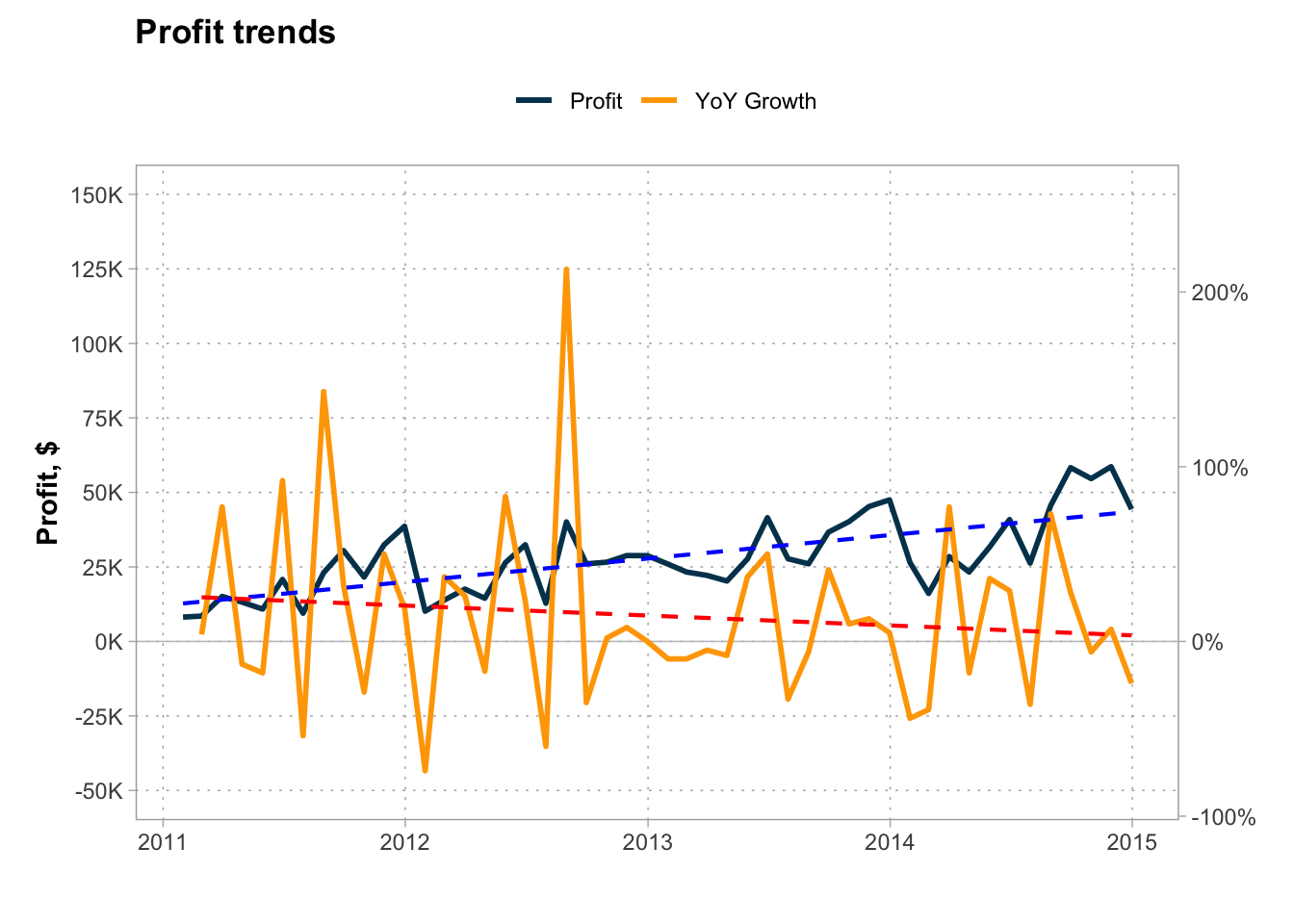
Total number of orders and loss orders
SELECT market,
             year,
             sum(sales) as sales,
             COUNT(DISTINCT order_id)::INT                               AS total_orders,
             (COUNT(DISTINCT order_id) FILTER ( WHERE profit < 0 ))::INT AS loss_orders
      FROM (SELECT market,
                   EXTRACT(YEAR FROM order_date) AS year,
                   order_id,
                   SUM(sales)                    AS sales,
                   SUM(profit)                   AS profit
            FROM analysis.all_global_orders
            GROUP BY 1, 2, 3) a
      GROUP BY 1, 2
ORDER BY 2, 3 descVisualize data for 2014 year.
ggplot(orders[orders$year == 2014, ]) +
  geom_col(
    aes(
      reorder(market, sales, decreasing = TRUE),
      sales, fill = "Revenue"
    ),
    position = "dodge2", show.legend = TRUE, alpha = 0.9
  ) +
  geom_segment(
    aes(
      x = reorder(market, sales),
      y = 0, xend = reorder(market, sales),
      yend = total_orders * 1e+06/max(orders[orders$year == 2014, ]$total_orders),
      color = "Total Orders"
    ),
    linetype = "solid"
  ) +
  geom_point(
    aes(
      reorder(market, sales, decreasing = TRUE),
      total_orders * 1e+06/max(orders[orders$year == 2014, ]$total_orders)
    ),
    shape = 95, size = 3, color = "black"
  ) +
  geom_col(
    aes(
      reorder(market, sales, decreasing = TRUE),
      loss_orders * 1e+06/max(orders[orders$year == 2014, ]$total_orders),
      fill = "Loss Orders"
    ),
    width = 0.1
  ) +
  scale_fill_manual(
    name = "", values = c(Revenue = "#ececec", `Loss Orders` = "red")
  ) +
  scale_color_manual(name = "", values = c(`Total Orders` = "black")) +
  theme(
    axis.text.x = element_text(color = "gray12", size = 12),
    legend.position = "top", panel.background = element_rect(fill = "white", color = "white")
  ) +
  scale_y_continuous(
    labels = scales::label_number(accuracy = 0.01, scale = 1e-06, suffix = "M"),
    limits = c(
      0, max(orders[orders$year == 2014, ]$sales) *
        1.1
    ),
    expand = c(0, 0),
    breaks = seq(
      0, max(orders[orders$year == 2014, ]$sales) *
        1.1, 250000
    ),
    sec.axis = sec_axis(
      trans = ~./1e+06 * max(orders[orders$year == 2014, ]$total_orders),
      name = "Number of Orders", breaks = seq(0, 2000, 250)
    )
  ) +
  labs(
    title = "Number of loss orders for 2014", y = "Revenue, $",
    x = "Market"
  ) +
  guides(
    color = guide_legend(override.aes = list(fill = "white")),
    linetype = guide_legend(override.aes = list(fill = "white"))
  )
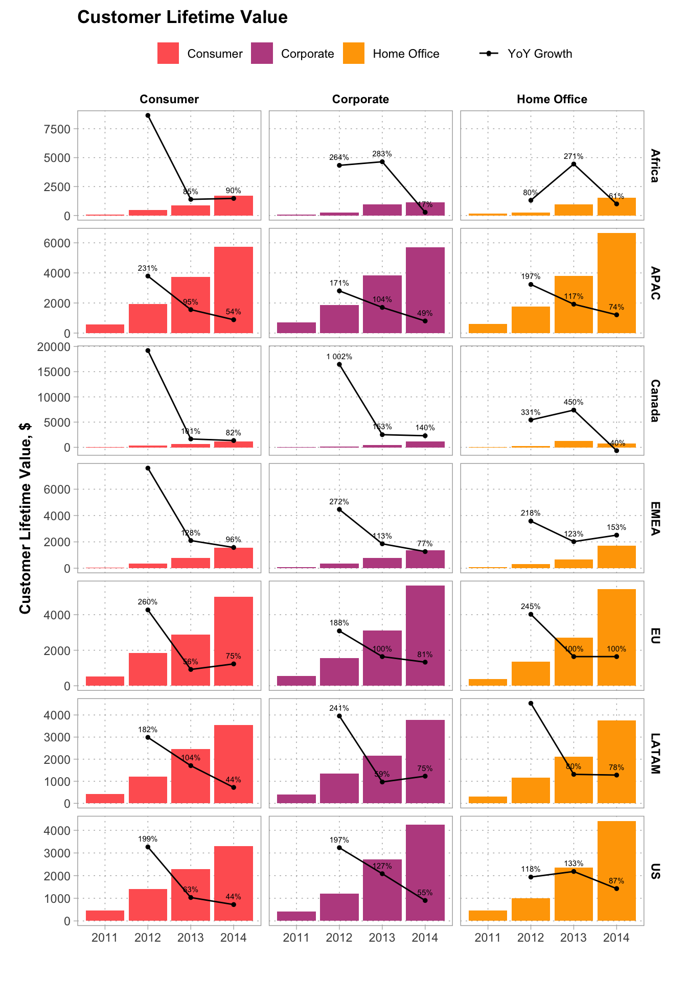
Customer Lifetime Value (CLV)
SELECT market,
       segment,
       year,
       round(CLV, 2) AS CLV,
       round((CLV - lag(CLV) OVER (PARTITION BY market, segment ORDER BY year))/lag(CLV) OVER (PARTITION BY market, segment ORDER BY year), 2) AS growth
FROM
(SELECT a.market,
       a.segment,
       a.year,
       a.customer_value * b.CLS AS CLV
  FROM (SELECT a.market,
               a.segment,
               a.year,
               a.sales,
               b.unique_customers,
               a.sales / b.unique_customers AS customer_value
        FROM (SELECT market,
                     segment,
                     EXTRACT(YEAR FROM order_date) AS year,
                     SUM(sales)                    AS sales
              FROM analysis.all_global_orders
              GROUP BY 1, 2, 3
              ORDER BY 1, 2, 3) a
                 LEFT JOIN
             (SELECT market,
                     segment,
                     EXTRACT(YEAR FROM order_date) AS year,
                     COUNT(DISTINCT customer_id)   AS unique_customers
              FROM analysis.all_global_orders
              GROUP BY 1, 2, 3
              ORDER BY 1, 2, 3) b ON a.market = b.market AND a.segment = b.segment AND a.year = b.year) a
           INNER JOIN
       (SELECT market,
               segment,
               year,
               DATE_PART('year', SUM(days))::decimal / COUNT(DISTINCT customer_id) AS CLS
        FROM (SELECT DISTINCT market,
                              segment,
                              year,
                              customer_id,
                              MIN(order_date) OVER (PARTITION BY customer_id)       AS first_date,
                              MAX(order_date) OVER (PARTITION BY year, customer_id) AS last_date,
                              AGE(MAX(order_date) OVER (PARTITION BY year, customer_id),
                                  MIN(order_date) OVER (PARTITION BY customer_id))  AS days

              FROM (SELECT *,
                           EXTRACT(YEAR FROM order_date) AS year
                    FROM analysis.all_global_orders) a) b
        GROUP BY 1, 2, 3) b ON
                   a.market = b.market AND
                   a.segment = b.segment AND
a.year = b.year) a;ggplot(CLV) +
geom_bar(
aes(x = year, y = clv, fill = segment),
stat = "identity", position = position_dodge()
) +
geom_line(
aes(
x = year, y = growth * mean(
CLV[CLV$market == market & CLV$segment ==
segment, "clv"]
),
color = "YoY Growth"
)
) +
geom_point(
aes(
x = year, y = growth * mean(
CLV[CLV$market == market & CLV$segment ==
segment, "clv"]
),
color = "YoY Growth"
),
size = 1
) +
geom_text(
aes(
x = year, y = growth * mean(
CLV[CLV$market == market & CLV$segment ==
segment, "clv"]
),
label = scales::percent(growth, accuracy = 1L),
color = "YoY Growth"
),
vjust = -1, size = 2
) +
labs(
title = "Customer Lifetime Value", x = "",
y = "Customer Lifetime Value, $"
) +
scale_fill_manual(
name = "", values = c(
Consumer = "#ff6361", Corporate = "#bc5090",
`Home Office` = "#ffa600"
)
) +
scale_color_manual(name = "", values = c(`YoY Growth` = "black")) +
facet_grid(market ~ segment, scales = "free_y") +
theme(
legend.position = "top", legend.title = element_blank(),
strip.background = element_blank(), strip.text = element_text(color = "black", face = "bold")
)
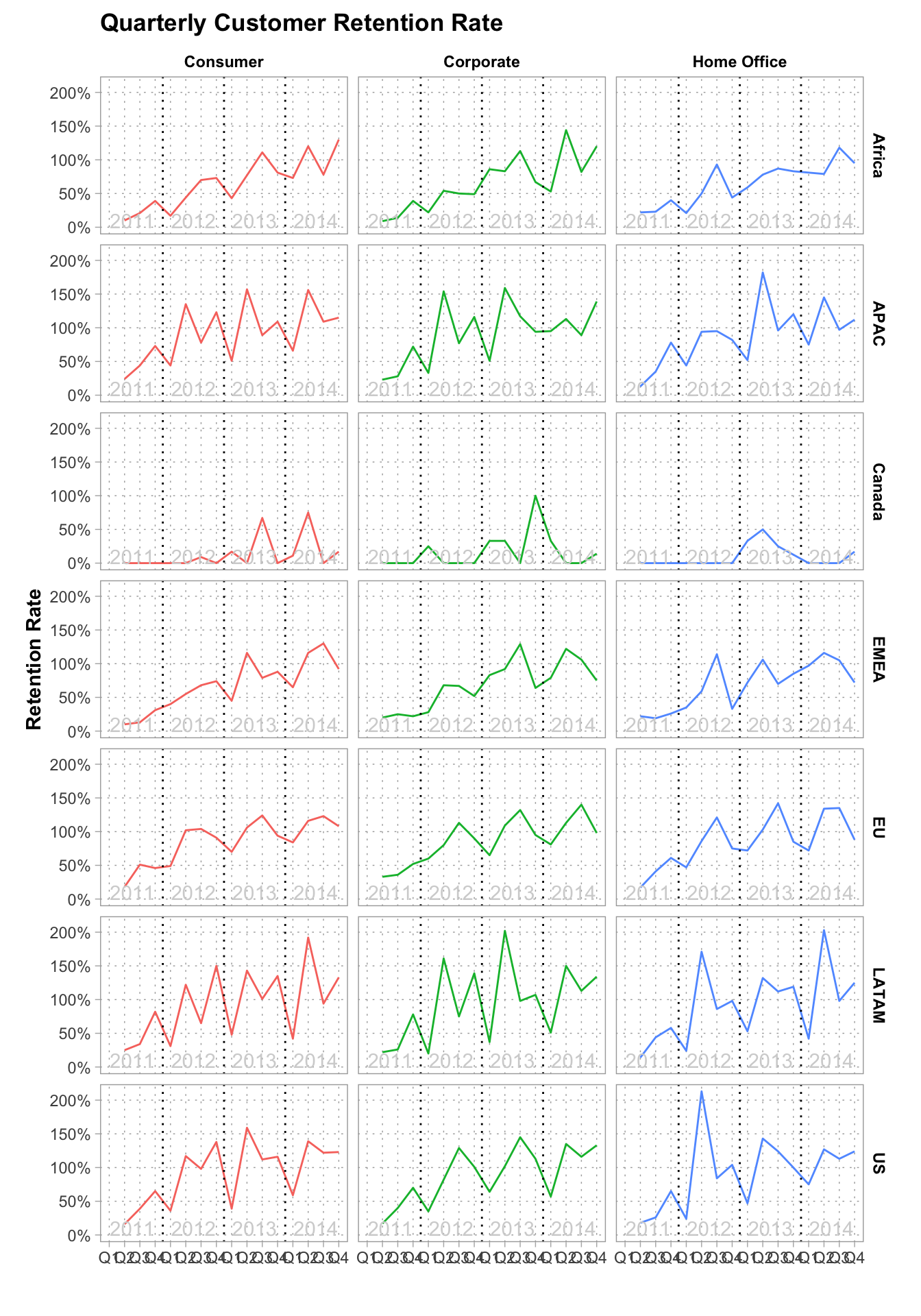
Quarterly Customer Retention Rate
WITH cte_orders AS (
SELECT DISTINCT
       order_id,
       customer_id,
       order_date,
       market,
       segment,
       min(order_date) OVER (PARTITION BY customer_id, market) AS first_date
FROM
    analysis.all_global_orders
ORDER BY customer_id, market, order_date),
    cte_orders_split AS (
SELECT *,
       extract(YEAR FROM order_date) AS order_year,
       extract(QUARTER FROM order_date) AS order_q,
       extract(YEAR FROM first_date) AS first_year,
       extract(QUARTER FROM first_date) AS first_q
FROM cte_orders)

SELECT year, quarter,
       market, segment,
       uniq_customers::INT,
       new_customers::INT,
       n::INT,
       CONCAT('Q', quarter, '''', SUBSTRING(TEXT(year), 3, 2))               AS qy,
       round((uniq_customers-coalesce(new_customers, 0))::decimal/lag(uniq_customers) OVER (PARTITION BY market, segment ORDER BY n), 2) AS ret_rate
FROM
(SELECT order_year AS year,
       order_q AS quarter,
       a.market,
       a.segment,
       a.uniq_customers,
       b.new_customers,
       row_number() OVER (PARTITION BY a.market, a.segment ORDER BY a.order_year, a.order_q) n
FROM
(SELECT order_year,
       order_q,
       market,
       segment,
       count(DISTINCT customer_id) uniq_customers
FROM cte_orders_split
GROUP BY 1, 2, 3, 4) a
LEFT JOIN
(SELECT first_year,
       first_q,
       market,
       segment,
       count(DISTINCT customer_id) new_customers
FROM cte_orders_split
GROUP BY 1, 2, 3, 4) b ON a.order_year = b.first_year AND
                          a.order_q = b.first_q AND
                          a.market = b.market AND
                          a.segment = b.segment
) a;ggplot(customer_retention) +
geom_line(
aes(
x = reorder(qy, n),
y = ret_rate, group = 1, color = segment
),
width = 2, show.legend = FALSE
) +
scale_y_continuous(labels = scales::label_percent()) +
geom_vline(
aes(xintercept = 4.5),
linetype = "dotted"
) +
geom_vline(
aes(xintercept = 8.5),
linetype = "dotted"
) +
geom_vline(
aes(xintercept = 12.5),
linetype = "dotted"
) +
annotate(
geom = "text", label = 2011, x = 2.5, y = 0.1,
color = "lightgray"
) +
annotate(
geom = "text", label = 2012, x = 6.5, y = 0.1,
color = "lightgray"
) +
annotate(
geom = "text", label = 2013, x = 10.5, y = 0.1,
color = "lightgray"
) +
annotate(
geom = "text", label = 2014, x = 14.5, y = 0.1,
color = "lightgray"
) +
scale_x_discrete(
labels = rep(
paste0("Q", 1:4),
4
)
) +
facet_grid(market ~ segment) +
theme(
legend.position = "top", legend.title = element_blank(),
strip.background = element_blank(), strip.text = element_text(color = "black", face = "bold")
) +
labs(
title = "Quarterly Customer Retention Rate",
x = "", y = "Retention Rate"
)
ARPPU and Average check value
SELECT (date_trunc('month', order_date))::date AS last_month_day,
       count(DISTINCT customer_id)::INT AS uniq_customers,
       count(DISTINCT order_id)::INT AS count_orders,
       round(sum(sales)/count(DISTINCT customer_id), 2) AS arppu,
       round(sum(sales)/count(DISTINCT order_id), 2) AS avg_check
FROM analysis.all_global_orders -- from materialized view
GROUP BY 1
ORDER BY 1;ggplot(arppu_check) +
geom_bar(
aes(x = last_month_day, y = arppu, fill = "ARPPU"),
stat = "identity"
) +
geom_line(
aes(
x = last_month_day, y = avg_check, color = "Avg. check"
),
size = 1
) +
geom_point(
aes(
x = last_month_day, y = avg_check, color = "Avg. check"
),
shape = 18, size = 3
) +
geom_smooth(
aes(x = last_month_day, y = avg_check),
method = "lm", color = "red", linetype = "dashed",
se = FALSE
) +
geom_smooth(
aes(x = last_month_day, y = arppu),
method = "lm", color = "blue", linetype = "dashed",
se = FALSE
) +
labs(
title = "Average revenue per paying user (ARPPU) and average check value\nfrom 2011 to 2014",
y = "ARPPU & Avg.check value, $", x = ""
) +
scale_fill_manual(name = "", values = c(ARPPU = "#003f5c")) +
scale_color_manual(name = "", values = c(`Avg. check` = "#ffa600")) +
theme(legend.position = "top")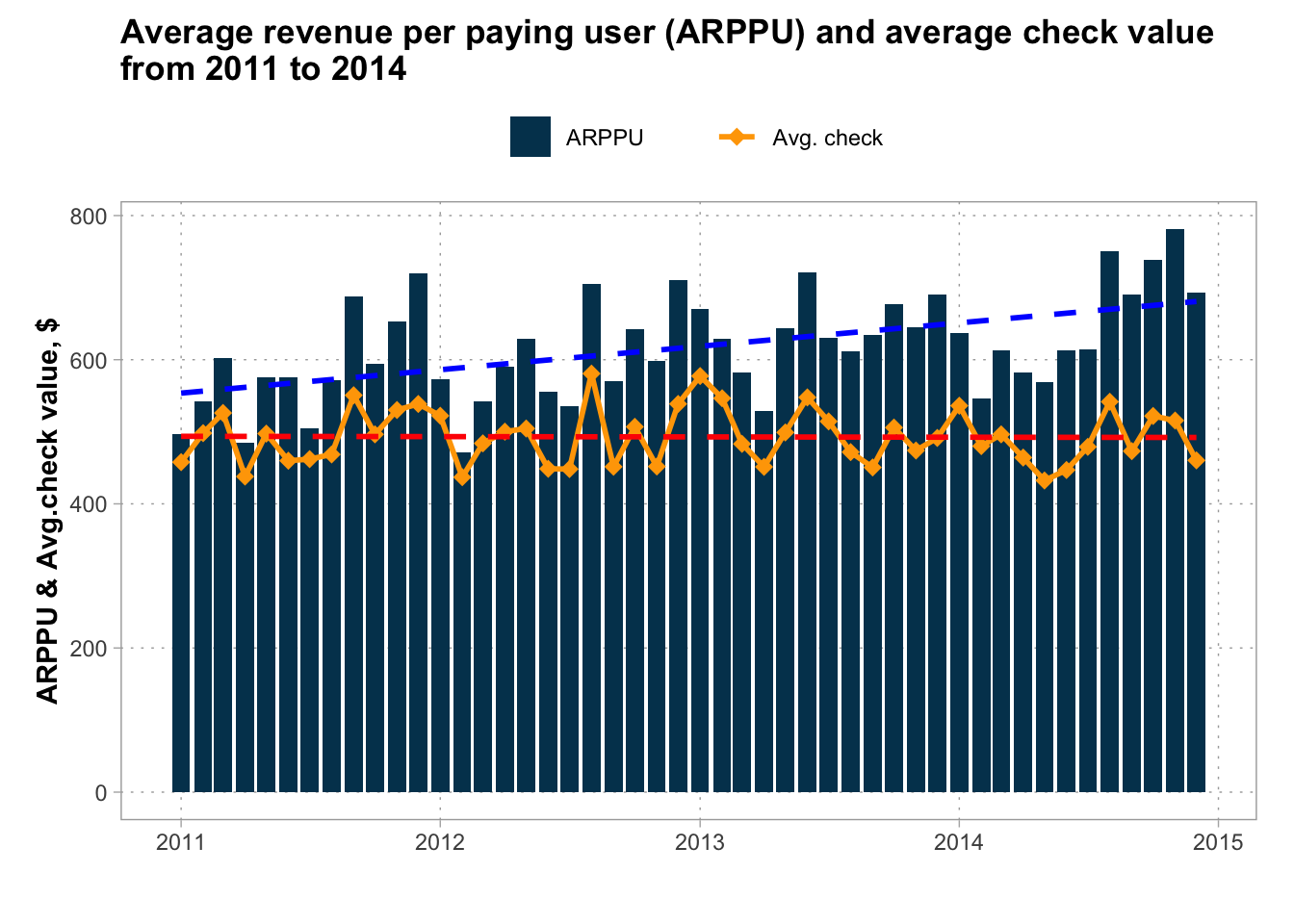
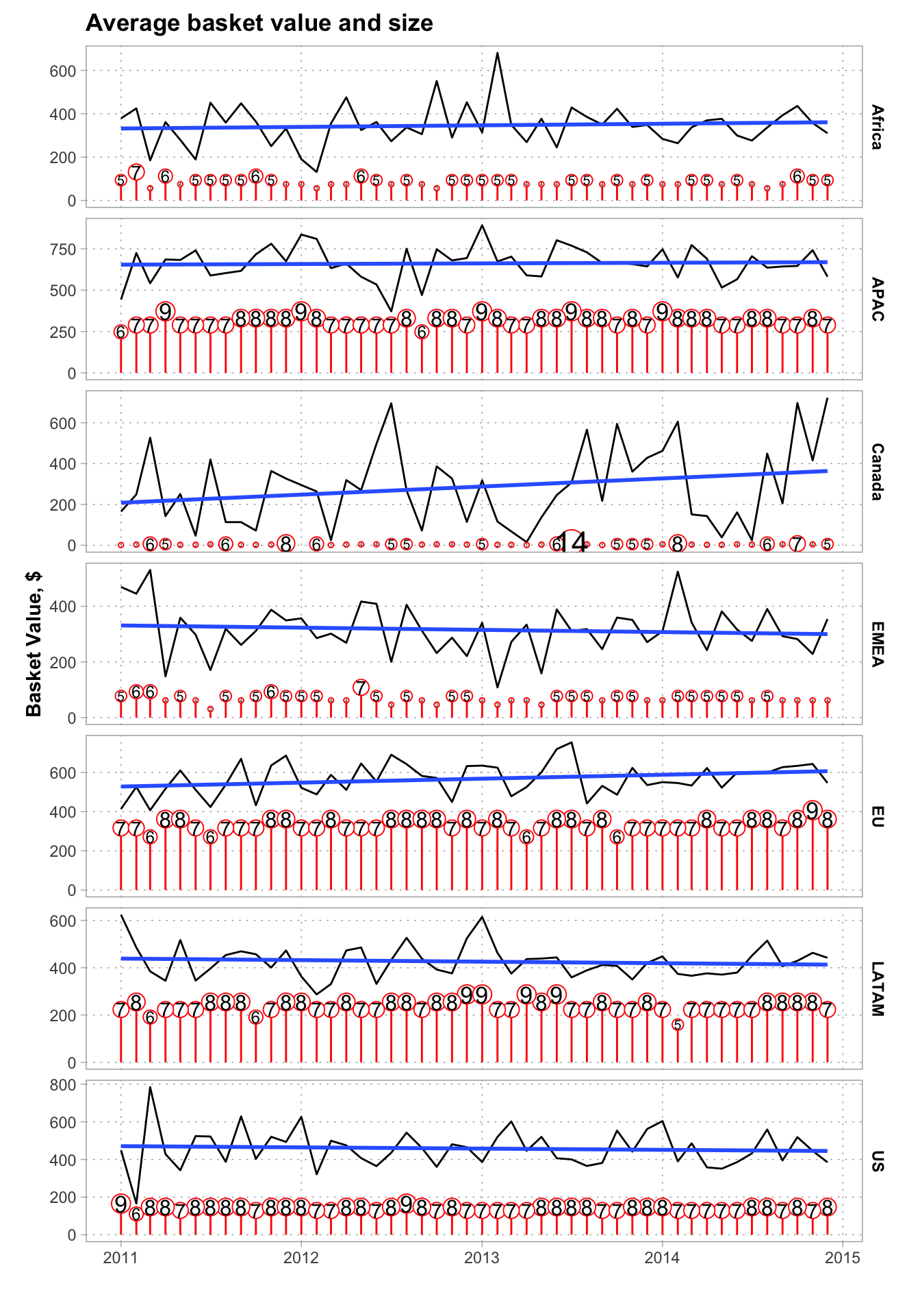
Average Basket Value and size
-- avg basket value and size
WITH order_cost AS (
    SELECT market,
       (date_trunc('month', order_date))::date AS last_month_day,
       segment,
       order_id,
       round(sum(sales), 2) as sales,
       round(sum(quantity), 2) as quantity
    FROM analysis.all_global_orders
    GROUP BY 1, 2, 3, 4
    ORDER BY 2, 1, 3, 4
    )


select *,
       round(min(basket_value) over (partition by market) / max(basket_size) over (partition by market), 2) AS scale
       from
(SELECT
    market,
    last_month_day,
    round(avg(sales), 2) AS basket_value,
    round(avg(quantity), 0) AS basket_size
    FROM order_cost
GROUP BY 1, 2) a;ggplot(basket_value) +
geom_line(
aes(
x = last_month_day, y = basket_value, group = market
)
) +
geom_segment(
aes(
x = last_month_day, xend = last_month_day,
y = 0, yend = basket_size * scale
),
color = "red"
) +
geom_point(
aes(
x = last_month_day, y = basket_size * scale,
size = ifelse(
basket_size <= 3, 2, basket_size -
2
)
),
shape = 21, color = "red", fill = "white",
show.legend = FALSE
) +
geom_text(
aes(
x = last_month_day, y = basket_size * scale,
label = basket_size, size = ifelse(
basket_size <= 3, 2, basket_size -
2
)
),
color = "black", show.legend = FALSE
) +
geom_smooth(
aes(x = last_month_day, y = basket_value),
method = "lm", se = FALSE, size = 1
) +
facet_grid(market ~ ., scales = "free_y") +
theme(
legend.position = "top", legend.title = element_blank(),
strip.background = element_blank(), strip.text = element_text(color = "black", face = "bold")
) +
labs(
title = "Average basket value and size", x = "",
y = "Basket Value, $"
)
Return Rate
-- return rate
SELECT extract(year from order_date) AS year,
       round(sum(sales), 2) AS total_sales,
       round(sum(sales) FILTER (WHERE returned), 2) AS returned_sales,
       count(distinct order_id)::INT AS count_orders,
       (count(distinct order_id) FILTER (WHERE returned))::INT AS returned_orders,
       round((count(distinct order_id) FILTER (WHERE returned))::decimal/count(distinct order_id), 3) as return_rate
FROM analysis.all_global_orders
GROUP BY 1;ggplot(returns) +
geom_bar(
aes(x = year, y = total_sales, fill = "Sales"),
stat = "identity", position = position_dodge(width = 0.8)
) +
geom_bar(
aes(
x = year, y = returned_sales, fill = "Returned Sales"
),
stat = "identity", position = position_dodge(width = 0.8)
) +
geom_point(
aes(
x = year, y = return_rate * total_sales,
color = "Return Rate"
)
) +
geom_text(
aes(
x = year, y = return_rate * total_sales,
label = scales::percent(return_rate, accuracy = 0.1)
),
vjust = -1.5
) +
labs(title = "Return rate", y = "Sales, $", x = "") +
scale_y_continuous(
labels = scales::label_number(scale = 1e-06, suffix = "M")
) +
scale_fill_manual(
name = "", values = c(Sales = "#dbe5da", `Returned Sales` = "#bbcbbc")
) +
scale_color_manual(name = "", values = c(`Return Rate` = "black")) +
theme(legend.position = "top")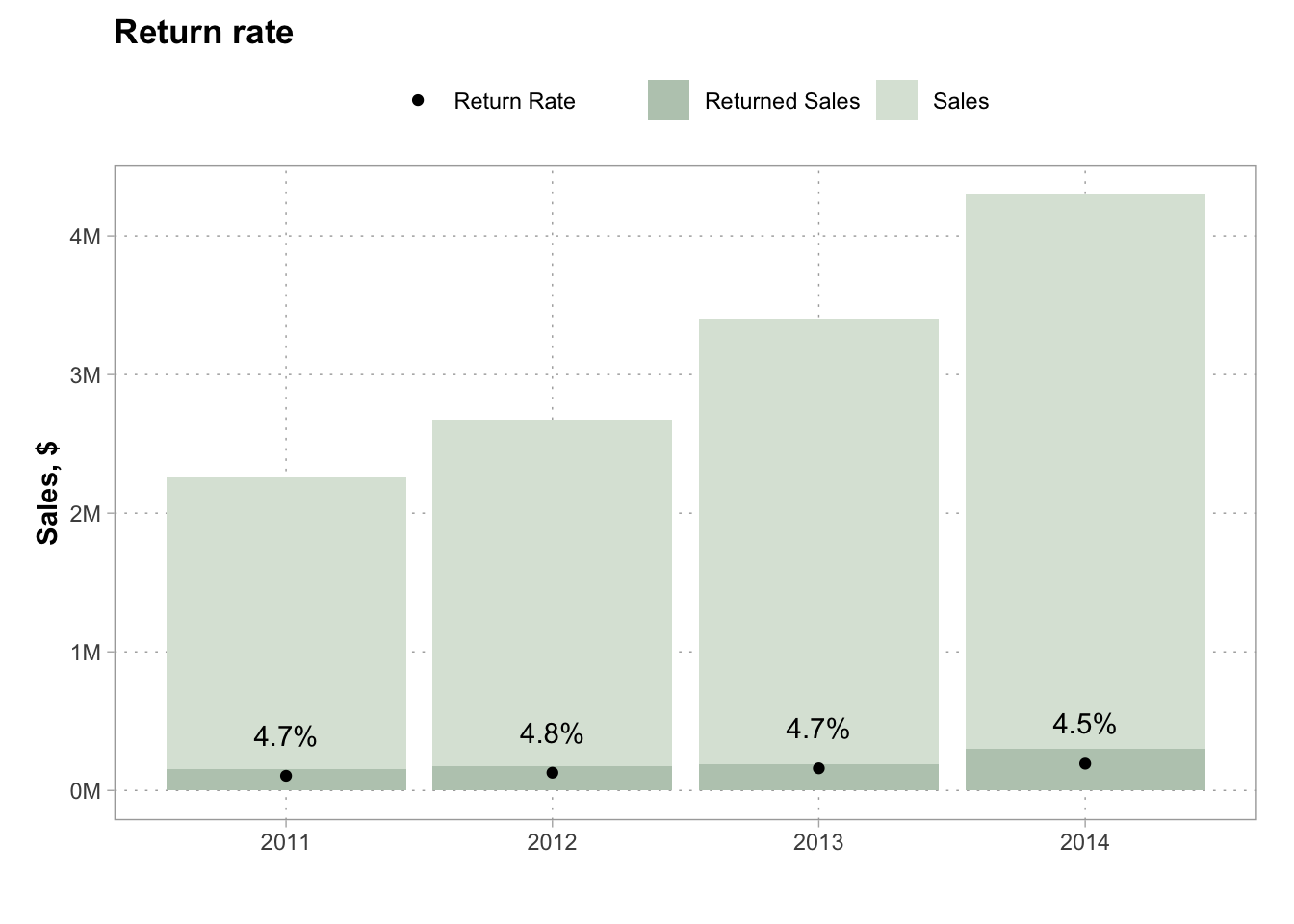
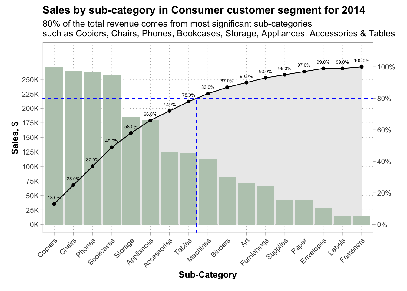
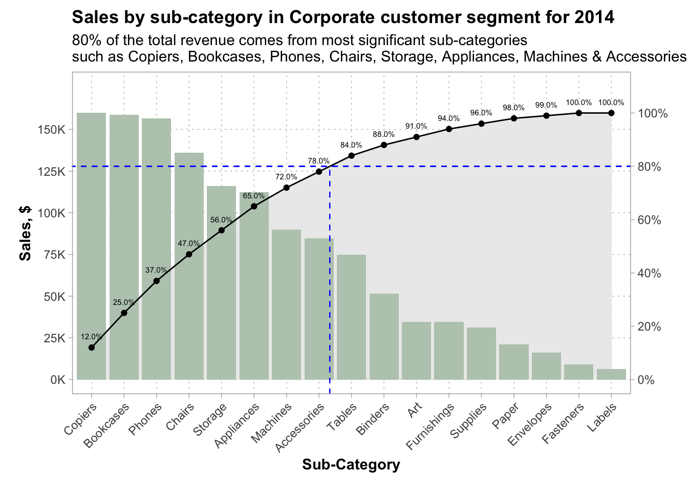
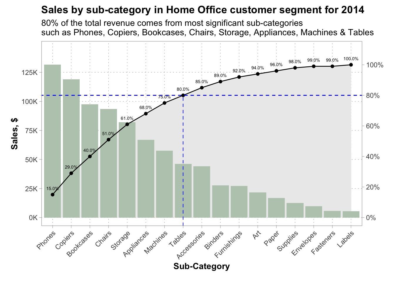
What most significant sub-categories?
WITH cte_sales AS(
SELECT extract(year from order_date) as year,
       sub_category,
       segment,
       sum(sales) as sales,
       sum(profit) as profit
from analysis.all_global_orders
group by 1, 2, 3)

select *,
       round(sum(sales/total_sales) over(partition by year, segment order by sales desc rows BETWEEN
            unbounded preceding and current row), 2) as cum_percent
       from
(select year, sub_category, segment,
       sales, sum(sales) over (PARTITION BY year, segment) as total_sales
from cte_sales
order by 1, 2, 3, 4 desc) a;for (segment in unique(pareto_sales$segment)) {
scale <- max(
pareto_sales[pareto_sales$year == 2014 & pareto_sales$segment ==
segment, ]$sales
)
x_intercept <- approx(
pareto_sales[pareto_sales$year == 2014 & pareto_sales$segment ==
segment, ]$cum_percent * scale, fct_reorder(
pareto_sales[pareto_sales$year == 2014 &
pareto_sales$segment == segment, ]$sub_category,
-pareto_sales[pareto_sales$year == 2014 &
pareto_sales$segment == segment, ]$sales
),
0.8 * scale
)$y
g <- ggplot(
pareto_sales[pareto_sales$year == 2014 & pareto_sales$segment ==
segment, ]
) +
geom_area(
aes(
x = fct_reorder(sub_category, -sales),
y = cum_percent * scale, group = 1
),
fill = "#ececec"
) +
geom_bar(
aes(
x = fct_reorder(sub_category, -sales),
y = sales
),
stat = "identity", fill = "#bbcbbc"
) +
geom_line(
aes(
x = fct_reorder(sub_category, -sales),
y = cum_percent * scale, group = 1
)
) +
geom_point(
aes(
x = fct_reorder(sub_category, -sales),
y = cum_percent * scale
)
) +
geom_text(
aes(
x = fct_reorder(sub_category, -sales),
y = cum_percent * scale, label = scales::percent(cum_percent, accuracy = 0.1)
),
size = 2, vjust = -1.5
) +
scale_y_continuous(
sec.axis = sec_axis(
trans = ~./scale, labels = scales::label_percent(),
breaks = seq(0, 1, 0.2)
),
breaks = seq(0, scale, 25000),
limits = c(0, scale * 1.1),
labels = scales::label_number(scale = 0.001, suffix = "K")
) +
scale_x_discrete(guide = guide_axis(angle = 45)) +
geom_segment(
x = 0, xend = Inf, y = 0.8 * scale, yend = 0.8 *
scale, color = "blue", size = 0.25,
linetype = "dashed"
) +
geom_segment(
x = x_intercept, xend = x_intercept, y = -Inf,
yend = 0.8 * scale, color = "blue", size = 0.25,
linetype = "dashed"
) +
labs(
title = paste0(
"Sales by sub-category in ", segment,
" customer segment for 2014"
),
x = "Sub-Category", y = "Sales, $", subtitle = paste0(
"80% of the total revenue comes from most significant sub-categories\nsuch as ",
stri_replace_last(
paste(
as.character(
fct_reorder(
pareto_sales[pareto_sales$year ==
2014 & pareto_sales$segment ==
segment, ]$sub_category,
-pareto_sales[pareto_sales$year ==
2014 & pareto_sales$segment ==
segment, ]$sales
)[seq(
1, round(8.27, 0),
1
)]
),
collapse = ", "
),
fixed = ",", " &"
)
)
)
print(g)
}
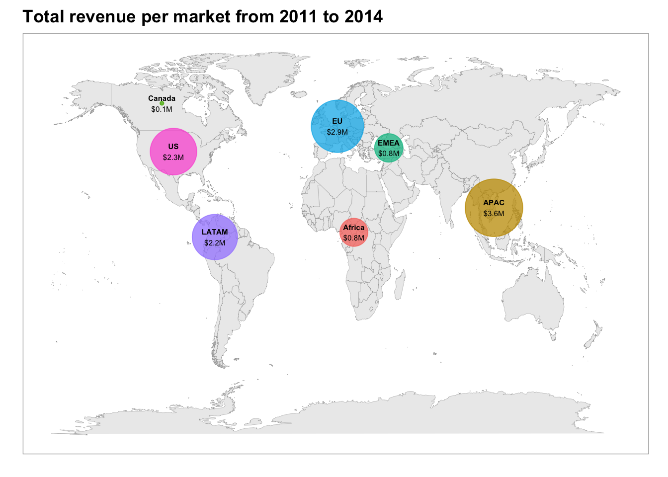
Map
SELECT market,
       region,
       country,
       sum(sales) AS sales
FROM analysis.all_global_orders
GROUP BY 1, 2, 3
ORDER BY 1, 2, 3;
# add geocodes
world <- map_data("world")
mapp <- map %>%
geocode(
country = country, method = "osm", lat = latitude,
long = longitude
)
centroids <- mapp %>%
group_by(market) %>%
summarise(
longitude = mean(longitude, na.rm = TRUE),
latitude = mean(latitude, na.rm = TRUE),
sales = sum(sales, na.rm = TRUE)
)
ggplot() + geom_map(
data = world, map = world, aes(long, lat, map_id = region),
color = "darkgray", fill = "#ececec", size = 0.1
) +
geom_point(
data = centroids, aes(
x = longitude, y = latitude, size = sales,
color = market
),
show.legend = FALSE, alpha = 0.75
) +
scale_size(range = c(1, 20)) +
geom_text(
data = centroids, aes(
x = longitude, y = latitude, label = scales::dollar(
sales, scale = 1e-06, suffix = "M",
accuracy = 0.1
)
),
size = 2, vjust = 1.5
) +
geom_text(
data = centroids, aes(x = longitude, y = latitude, label = market),
size = 2, vjust = -0.5, fontface = "bold"
) +
labs(
title = "Total revenue per market from 2011 to 2014",
x = "", y = ""
) +
theme(
axis.line = element_blank(), axis.text.x = element_blank(),
axis.text.y = element_blank(), axis.ticks = element_blank(),
axis.title.x = element_blank(), axis.title.y = element_blank(),
legend.position = "none", panel.background = element_blank(),
panel.grid.major = element_blank(), panel.grid.minor = element_blank(),
plot.background = element_blank()
)
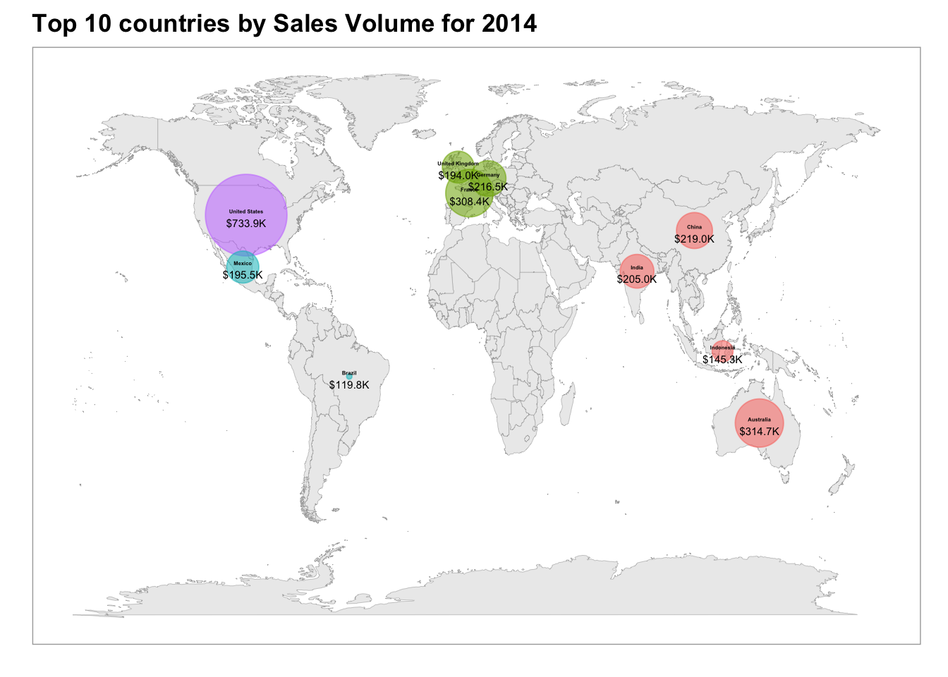
Top 10 countries by Sales Volume
select * from
(select *,
       round((sales - lag(sales) over (PARTITION BY market, country  ORDER BY year))/
       lag(sales) over (PARTITION BY market, country  ORDER BY  year), 2) as YoY_Growth_Sales,
       round((profit - lag(profit) over (PARTITION BY market, country  ORDER BY year))/
       lag(profit) over (PARTITION BY market, country  ORDER BY  year), 2) as YoY_Growth_Profit
from
(select market,
       country,
       extract(year from order_date) as year,
       sum(sales) as sales,
       sum(profit) as profit
from analysis.all_global_orders
group by 1, 2, 3) a) a
where year = 2014 ORDER BY sales desc limit 10;top_sales_countries %>%
mutate_at(
c("yoy_growth_sales", "yoy_growth_profit"),
~cell_spec(
scales::percent(., accuracy = 0.1),
"html", color = case_when(
. < 0 ~ "red", . >= 0 ~ "green", is.na(.) ~
"lightgray", TRUE ~ "black"
)
)
) %>%
mutate_at(
c("sales", "profit"),
~scales::dollar(., accuracy = 0.01)
) %>%
relocate(yoy_growth_sales, .after = sales) %>%
select(-year) %>%
kbl(
col.names = c(
"Market", "Country", "Total", "YoY Growth",
"Total", "YoY Growth"
),
caption = "Top 10 countries by Sales Volume for 2014",
escape = F, align = c("llrrrr")
) %>%
row_spec(0, align = "c") %>%
kable_styling(
bootstrap_options = c("striped", "bordered"),
full_width = TRUE
) %>%
add_header_above(
header = c(" ", " ", Sales = 2, Profit = 2),
bold = TRUE, border_left = TRUE, border_right = TRUE
)| Market | Country | Total | YoY Growth | Total | YoY Growth |
|---|---|---|---|---|---|
| US | United States | $733,946.97 | 21.0% | $93,507.97 | 14.0% |
| APAC | Australia | $314,733.41 | 17.0% | $32,030.37 | 11.0% |
| EU | France | $308,437.39 | 34.0% | $35,142.08 | 8.0% |
| APAC | China | $218,979.31 | 12.0% | $46,793.98 | 5.0% |
| EU | Germany | $216,537.21 | 47.0% | $35,956.07 | 33.0% |
| APAC | India | $205,032.00 | 35.0% | $48,807.66 | 48.0% |
| LATAM | Mexico | $195,479.76 | 23.0% | $31,330.88 | 12.0% |
| EU | United Kingdom | $194,005.10 | 56.0% | $36,755.55 | 33.0% |
| APAC | Indonesia | $145,334.84 | 40.0% | $10,527.21 | 1 124.0% |
| LATAM | Brazil | $119,772.15 | 29.0% | $15,422.79 | 681.0% |
countries_coords <- top_sales_countries %>%
  geocode(
    country = country, method = "osm", lat = latitude,
    long = longitude
  )

ggplot() + geom_map(
  data = world, map = world, aes(long, lat, map_id = region),
  color = "darkgray", fill = "#ececec", size = 0.1
) +
  geom_point(
    data = countries_coords, aes(
      x = longitude, y = latitude, size = sales,
      color = market, alpha = 0.5
    ),
    show.legend = FALSE
  ) +
  scale_size(range = c(1, 20)) +
  geom_text(
    data = countries_coords, aes(
      x = longitude, y = latitude, label = scales::dollar(
        sales, scale = 0.001, suffix = "K",
        accuracy = 0.1
      )
    ),
    size = 2, vjust = 1.5
  ) +
  geom_text(
    data = countries_coords, aes(x = longitude, y = latitude, label = country),
    size = 1, vjust = -0.5, fontface = "bold"
  ) +
  labs(
    title = "Top 10 countries by Sales Volume for 2014",
    x = "", y = ""
  ) +
  theme(
    axis.line = element_blank(), axis.text.x = element_blank(),
    axis.text.y = element_blank(), axis.ticks = element_blank(),
    axis.title.x = element_blank(), axis.title.y = element_blank(),
    legend.position = "none", panel.background = element_blank(),
    panel.grid.major = element_blank(), panel.grid.minor = element_blank(),
    plot.background = element_blank()
  )
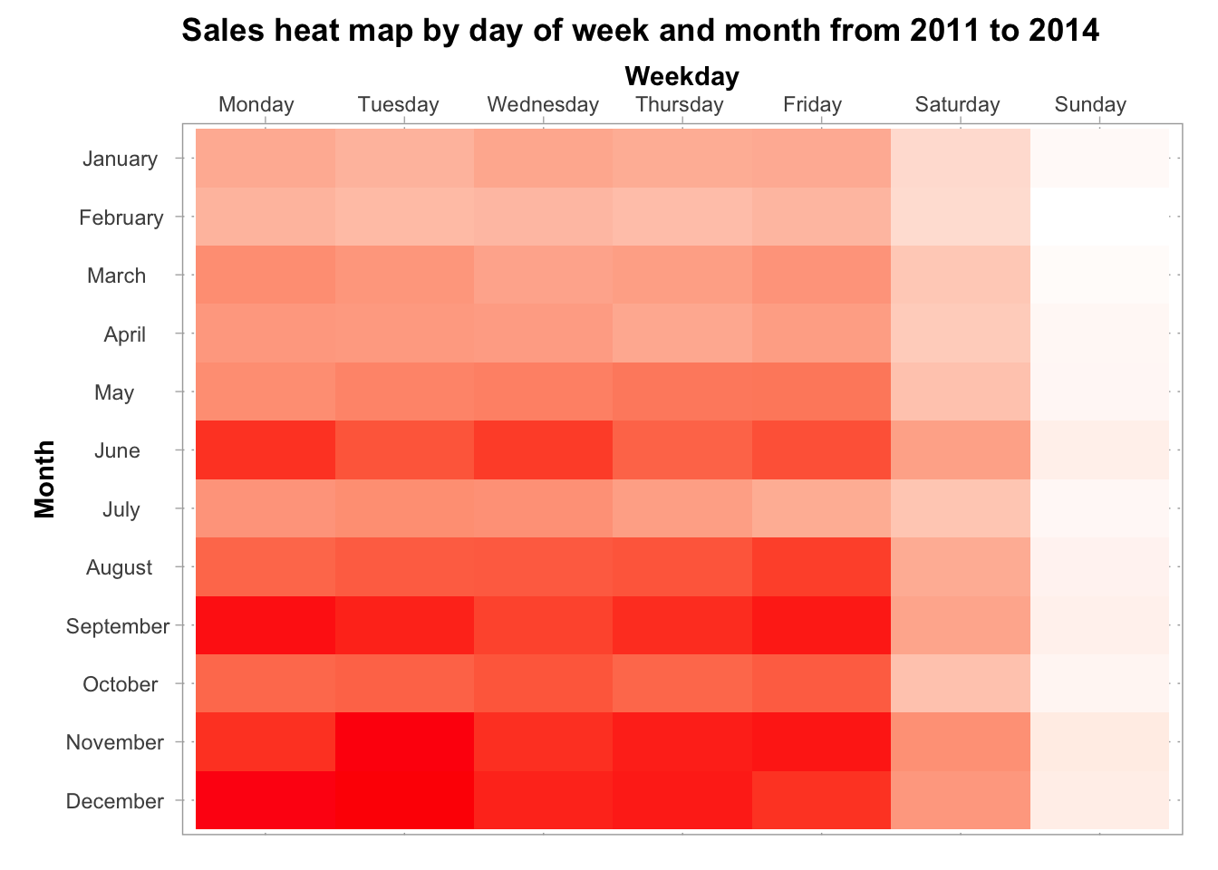
Sales analysis heat map by day and month
SELECT *,
       count_orders::numeric / (SUM(count_orders) OVER ()) AS proc
FROM (SELECT month,
             n_month,
             wod,
             n_wod,
             COUNT(DISTINCT order_id)::INT count_orders
      FROM (SELECT DISTINCT order_id,
                EXTRACT(MONTH FROM FIRST_VALUE(order_date) OVER (PARTITION BY order_id))  AS n_month,
                TO_CHAR(FIRST_VALUE(order_date) OVER (PARTITION BY order_id), 'Month')    AS month,
                EXTRACT(ISODOW FROM FIRST_VALUE(order_date) OVER (PARTITION BY order_id)) AS n_wod,
                TO_CHAR(FIRST_VALUE(order_date) OVER (PARTITION BY order_id), 'Day')      AS wod
            FROM analysis.all_global_orders
            ORDER BY n_month, n_wod) a
      GROUP BY month, n_month, wod, n_wod) a
ORDER BY n_month, n_wod;heat %>%
mutate(
wod = as.factor(wod),
month = as.factor(month)
) %>%
mutate(
wod = fct_reorder(wod, n_wod),
month = fct_reorder(month, -n_month)
) %>%
ggplot(aes(x = wod, y = month, fill = proc)) +
geom_tile(show.legend = FALSE) +
scale_fill_gradient(high = "red", low = "white", na.value = "white") +
scale_x_discrete(position = "top") +
labs(
title = "Sales heat map by day of week and month from 2011 to 2014",
x = "Weekday", y = "Month"
)
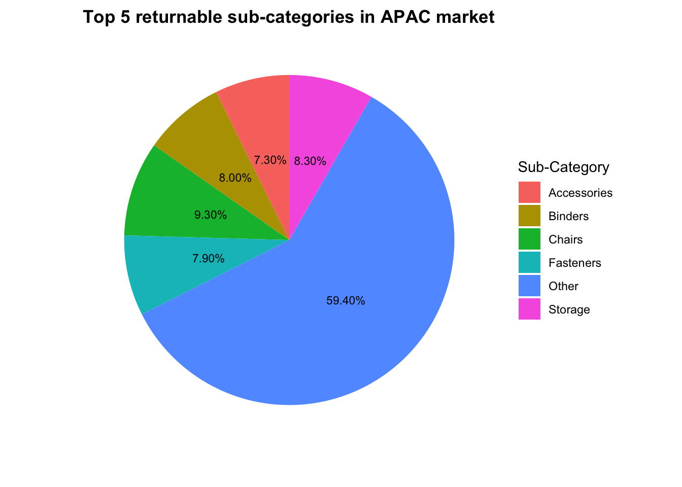
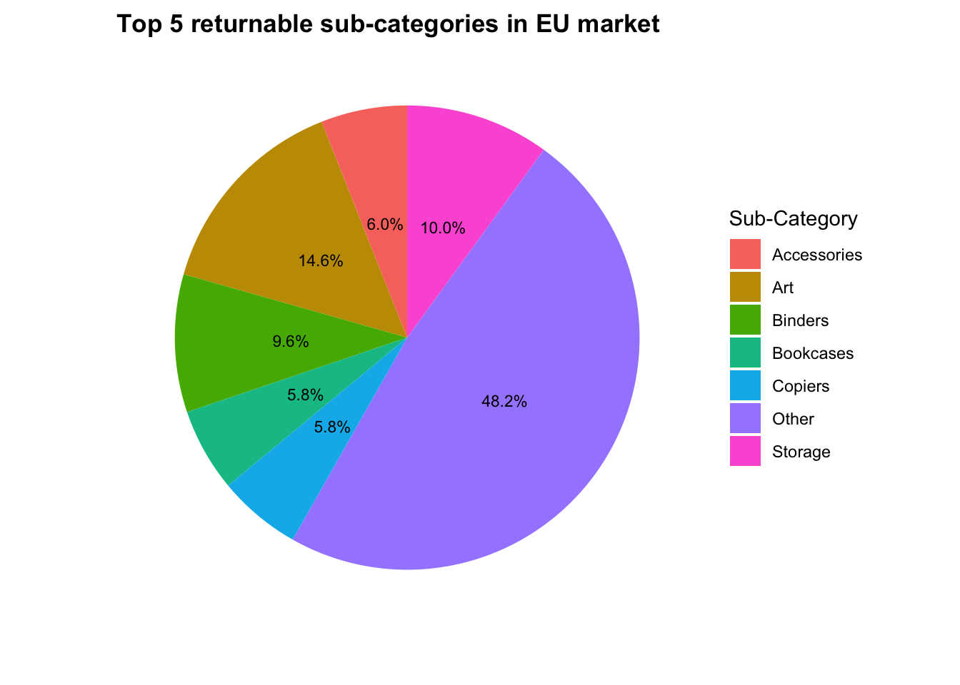
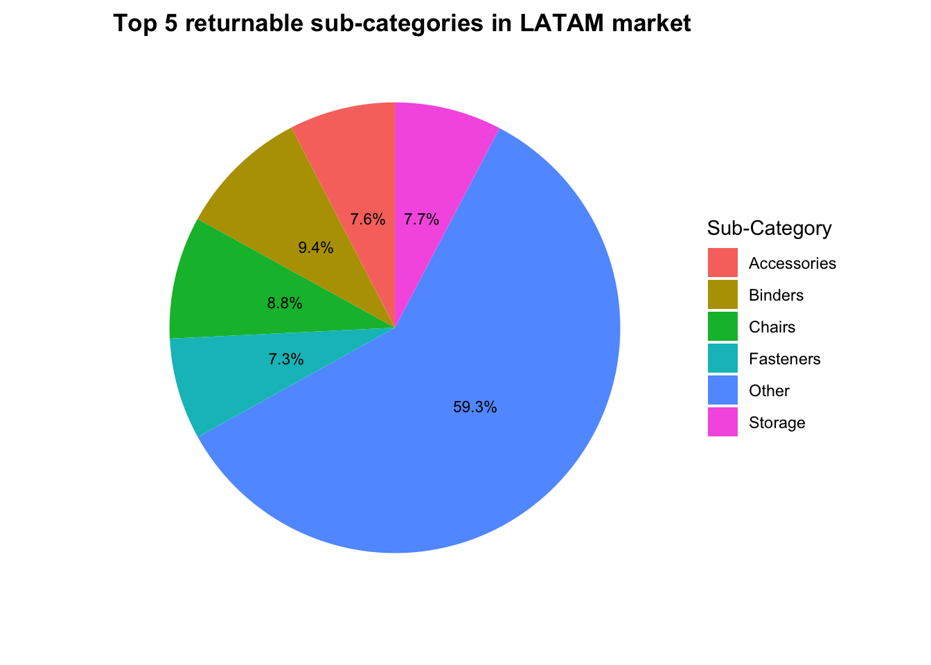
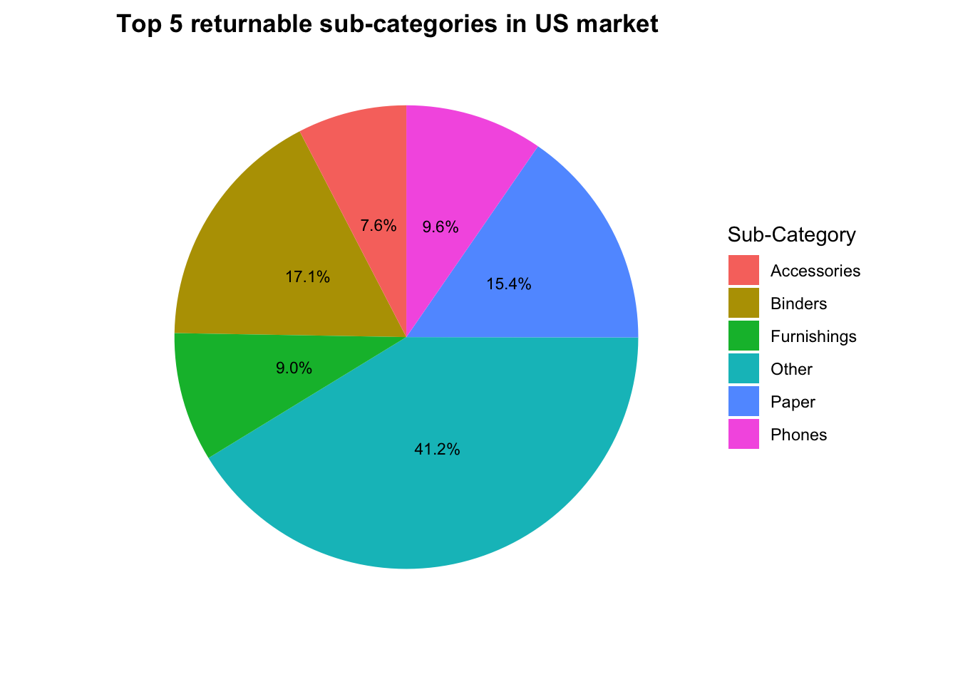
Top 5 returnable sub-categories by merket
SELECT a.market,
       a.new_sub_category AS sub_category,
       SUM(a.perc)        AS perc
FROM (SELECT a.market,
             a.perc,
             CASE
                 WHEN RANK() OVER (PARTITION BY market ORDER BY perc DESC) <= 5 THEN sub_category
                 ELSE 'Other'
                 END AS new_sub_category
      FROM (SELECT DISTINCT market,
                            sub_category,
                            ROUND(COUNT(*) OVER (PARTITION BY market, sub_category) /
                                  COUNT(*) OVER (PARTITION BY market)::numeric, 3) AS perc
            FROM analysis.all_global_orders
            WHERE returned
            ORDER BY market, perc DESC) a) a
GROUP BY market, sub_category
ORDER BY market, perc DESC;for (market in unique(returnable_sub_category$market)) {
print(
returnable_sub_category[returnable_sub_category$market ==
market, ] %>%
ggplot(aes(x = "", y = perc, fill = sub_category)) +
geom_col() + geom_text(
aes(label = scales::percent(perc)),
size = 3, position = position_stack(vjust = 0.5)
) +
coord_polar(theta = "y") +
labs(
title = paste(
"Top 5 returnable sub-categories in",
market, "market"
),
x = "", y = "", fill = "Sub-Category"
) +
theme(
axis.text = element_blank(), axis.ticks = element_blank(),
panel.grid = element_blank(), panel.grid.major = element_blank(),
panel.border = element_blank()
)
)
}
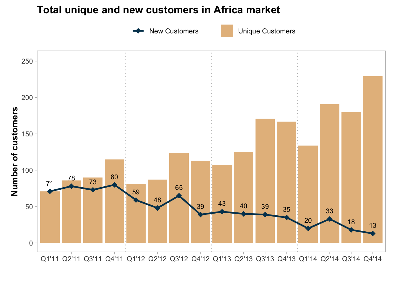
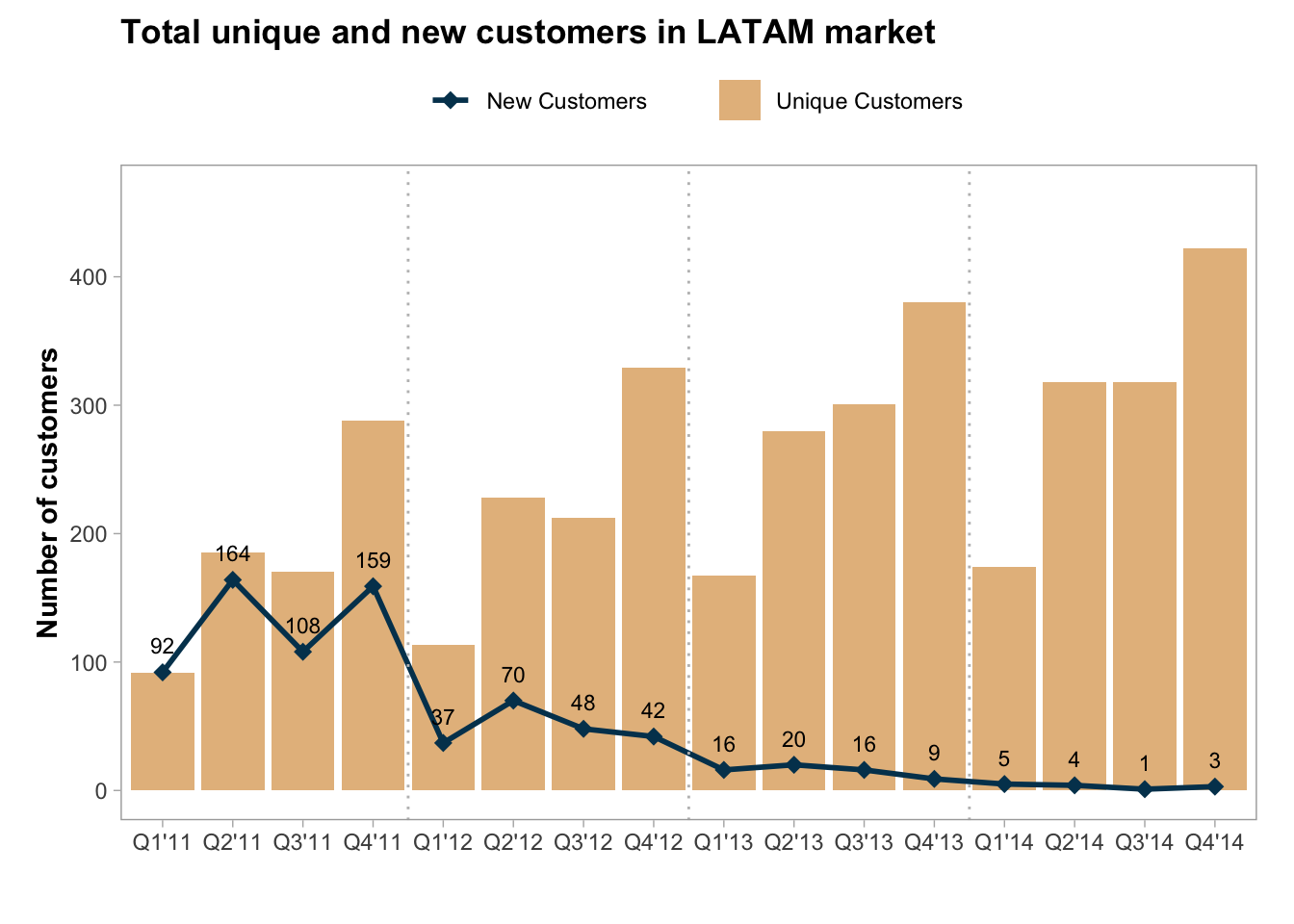
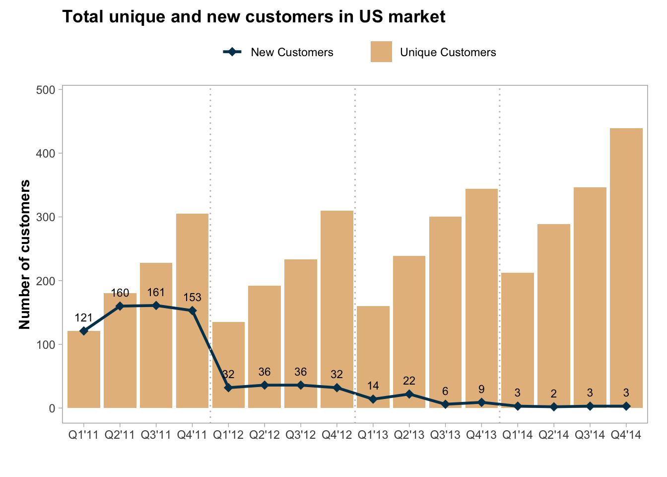
What are number of total and new customers?
WITH cte_timespot AS (SELECT m.market, a.year, a.quarter
                      FROM (SELECT DISTINCT market FROM analysis.all_global_orders) m
                               CROSS JOIN
                           (SELECT b.year, a.quarter
                            FROM (SELECT UNNEST(ARRAY [1, 2, 3, 4]) AS quarter) a
                                     CROSS JOIN
                                     (SELECT UNNEST(ARRAY [2011, 2012, 2013, 2014]) AS year) b
                            ORDER BY 1, 2) a
                      ORDER BY 1, 2, 3),
     cte_unique_customers AS (SELECT market,
                                     EXTRACT(YEAR FROM order_date)    AS year,
                                     EXTRACT(QUARTER FROM order_date) AS quarter,
                                     COUNT(DISTINCT customer_id)      AS unique_customers
                              FROM analysis.all_global_orders
                              GROUP BY 1, 2, 3),
     cte_new_customers AS (SELECT market,
                                  year,
                                  quarter,
                                  COUNT(DISTINCT customer_id) AS new_customers
                           FROM (SELECT DISTINCT market,
                                                 customer_id,
                                                 FIRST_VALUE(EXTRACT(YEAR FROM order_date))
                                                 OVER (PARTITION BY market, customer_id ORDER BY EXTRACT(YEAR FROM order_date))                                   AS year,
                                                 FIRST_VALUE(EXTRACT(QUARTER FROM order_date))
                                                 OVER (PARTITION BY market, customer_id ORDER BY EXTRACT(YEAR FROM order_date), EXTRACT(QUARTER FROM order_date)) AS quarter
                                 FROM analysis.all_global_orders) a
                           GROUP BY market, year, quarter)
SELECT a.market,
       a.year,
       a.quarter,
       a.unique_customers::INT,
       COALESCE(b.new_customers, 0)::INT AS new_customers,
       CONCAT('Q', a.quarter, '''', SUBSTRING(TEXT(a.year), 3, 2))               AS qy,
       ROW_NUMBER() OVER (PARTITION BY a.market ORDER BY a.year, a.quarter)::INT AS n
FROM cte_timespot t
         LEFT JOIN
     cte_unique_customers a ON t.market = a.market AND t.year = a.year AND t.quarter = a.quarter
         LEFT JOIN
cte_new_customers b ON a.market = b.market AND a.year = b.year AND a.quarter = b.quarter;for (market in unique(new_total_customers$market)) {
plot <- ggplot(
new_total_customers[new_total_customers$market ==
market, ]
) +
geom_bar(
aes(
x = fct_reorder(qy, n),
y = unique_customers, fill = "Unique Customers"
),
stat = "identity"
) +
geom_line(
aes(
x = fct_reorder(qy, n),
y = new_customers, group = 1, color = "New Customers"
),
size = 1
) +
geom_point(
aes(
x = fct_reorder(qy, n),
y = new_customers, color = "New Customers"
),
shape = 18, size = 3
) +
geom_text(
aes(
x = fct_reorder(qy, n),
y = new_customers, label = scales::number(new_customers)
),
size = 3, vjust = -1.2
) +
geom_vline(
xintercept = seq(4.5, 12.5, 4),
linetype = "dotted", color = "gray"
) +
scale_fill_manual(
name = "", values = c(`Unique Customers` = "#e5bc8b")
) +
scale_color_manual(
name = "", values = c(`New Customers` = "#003f5c")
) +
scale_y_continuous(
limits = c(
0, max(
new_total_customers[new_total_customers$market ==
market, ]$unique_customers
) *
1.1
)
) +
labs(
title = paste(
"Total unique and new customers in",
market, "market"
),
x = "", y = "Number of customers"
) +
theme(
legend.position = "top", panel.grid.major = element_blank()
)
print(plot)
}
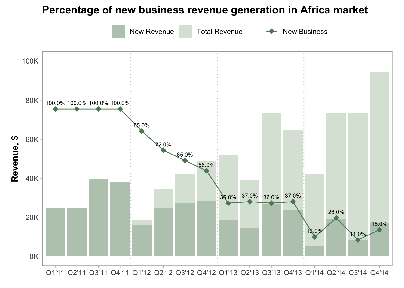
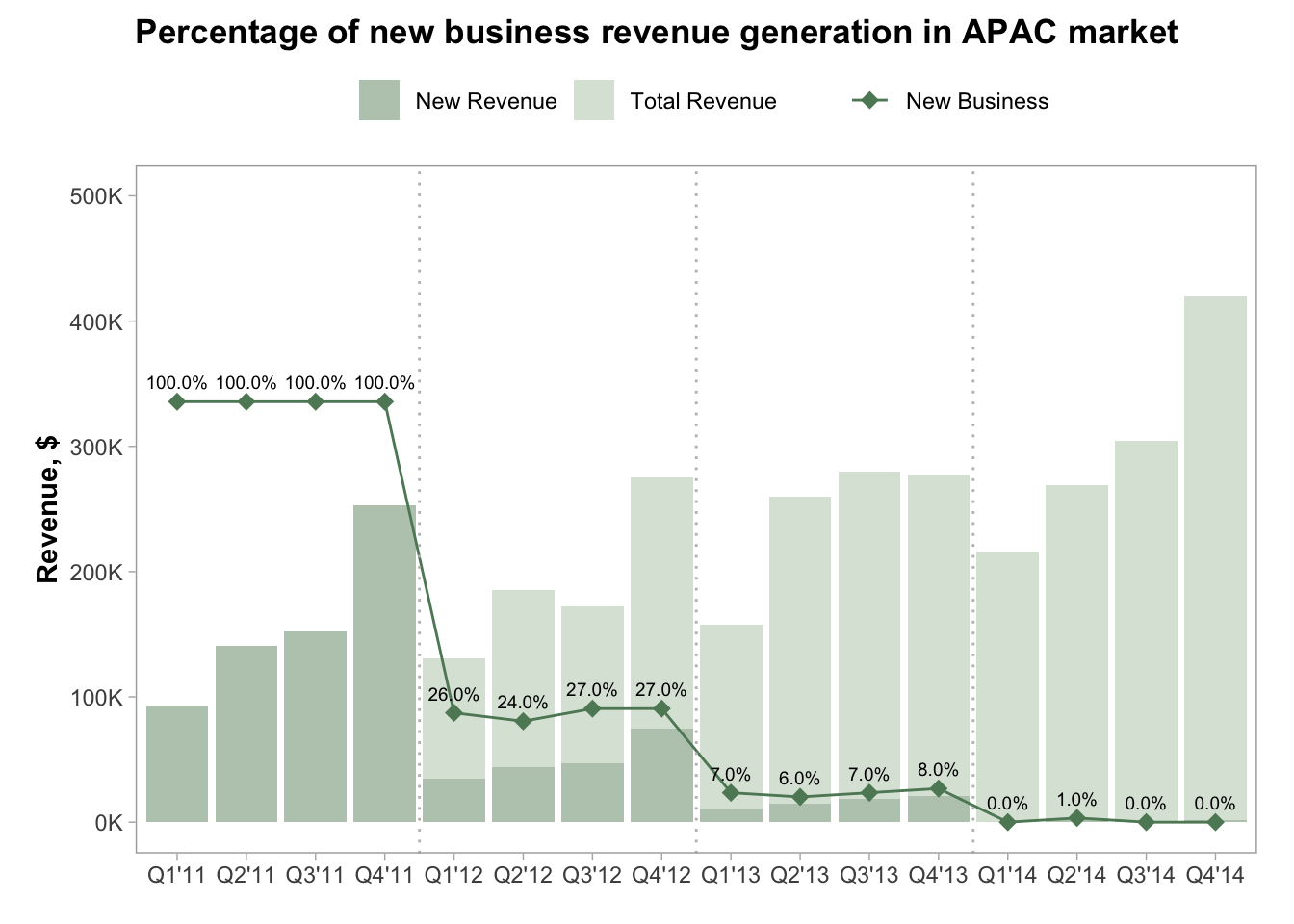
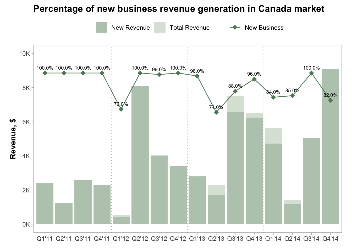
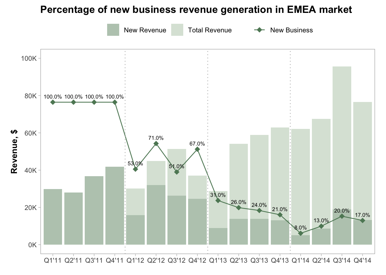
Percentage of new business revenue generation
WITH cte_all_orders AS (SELECT market,
                               order_id,
                               order_date,
                               customer_id,
                               SUM(sales) AS sales
                        FROM analysis.all_global_orders
                        GROUP BY 1, 2, 3, 4)
SELECT *,
       ROW_NUMBER() OVER (PARTITION BY market ORDER BY year, quarter) AS n
FROM (SELECT market,
             year,
             quarter,

             CONCAT('Q', quarter, '''', SUBSTRING(TEXT(year), 3, 2))                           AS qy,
             COALESCE(SUM(sales) FILTER (WHERE year = first_year), 0)                          AS new_sales,
             SUM(sales)                                                                        AS total_sales,
             ROUND((COALESCE(SUM(sales) FILTER (WHERE year = first_year), 0)) / SUM(sales), 2) AS proc_new_business
      FROM (SELECT *,
                   EXTRACT(YEAR FROM order_date)                               AS year,
                   EXTRACT(QUARTER FROM order_date)                            AS quarter,
                   FIRST_VALUE(EXTRACT(YEAR FROM order_date))
                   OVER (PARTITION BY market, customer_id ORDER BY order_date) AS first_year
            FROM cte_all_orders) a
GROUP BY market, year, quarter, qy) a;for (market in unique(new_business$market)) {
scale <- max(
new_business[new_business$market == market,
]$total_sales
)
hi <- round(
scale * 1.1/10^floor(log10(scale * 1.1)),
0
) *
10^floor(log10(scale * 1.1))
scale <- scale * 0.8
plot <- new_business[new_business$market == market,
] %>%
ggplot() + geom_bar(
aes(
x = fct_reorder(qy, n),
y = total_sales, fill = "Total Revenue"
),
stat = "identity"
) +
geom_bar(
aes(
x = fct_reorder(qy, n),
y = new_sales, fill = "New Revenue"
),
stat = "identity"
) +
geom_line(
aes(
x = fct_reorder(qy, n),
y = proc_new_business * scale, group = 1,
color = "New Business"
)
) +
geom_point(
aes(
x = fct_reorder(qy, n),
y = proc_new_business * scale, color = "New Business"
),
shape = 18, size = 3
) +
geom_text(
aes(
x = fct_reorder(qy, n),
y = proc_new_business * scale, label = scales::percent(proc_new_business, accuracy = 0.1)
),
shape = 18, size = 2.5, vjust = -1
) +
geom_vline(
xintercept = seq(4.5, 12.5, 4),
linetype = "dotted", color = "gray"
) +
scale_y_continuous(
limits = c(0, hi),
breaks = seq(0, hi, by = hi/5),
labels = scales::number(
seq(0, hi, by = hi/5),
scale = 10^-(floor(log10(hi)) -
floor(log10(hi))%%3),
suffix = ifelse(
floor(log10(hi)) -
floor(log10(hi))%%3 >
3, "M", "K"
)
)
) +
labs(
title = paste(
"Percentage of new business revenue generation in",
market, "market"
),
x = "", y = "Revenue, $"
) +
theme(
legend.position = "top", legend.title = element_blank(),
axis.title.x = element_blank(), panel.grid.major = element_blank()
) +
scale_fill_manual(
name = "", values = c(
`Total Revenue` = "#dbe5da", `New Revenue` = "#bbcbbc"
)
) +
scale_color_manual(
name = "", values = c(`New Business` = "#5e8765")
)
print(plot)
}