Chapter 5 ARMA processes

library(tidyverse)
library(fpp3)
library(ggplot2)
library(rio)

5.1 AR process

An \(\textbf{AR(p)}\) process is described by the following equation: \[ y_t = c + \beta_1 y_{t-1} + \ldots + \beta_p y_{t-p} + u_t, \] where \(u_t\) represents white noise, and \(\beta_p \neq 0\). This process is called a solution of the \(MA(\infty)\) relative to \(u_t\).

\(AR(p)\) process is stationary.

5.2 ARMA process

An \(\textbf{ARMA(p, q)}\) process is described by the following equation:

\[ y_t = c + \beta_1 y_{t-1} + \ldots + \beta_p y_{t-p} + u_t + \alpha_1 u_{t-1} + \ldots + \alpha_q u_{t-q}, \]

where \(u_t\) represents white noise, \(\beta_p \neq 0\), and \(\alpha_q \neq 0\). This process is called a solution of the \(MA(\infty)\) relative to \(u_t\).

5.3 Examples

set.seed(777)

# generate data
data <- tibble(a = arima.sim(n = 100,
                             model = list(ar = 0.5)),
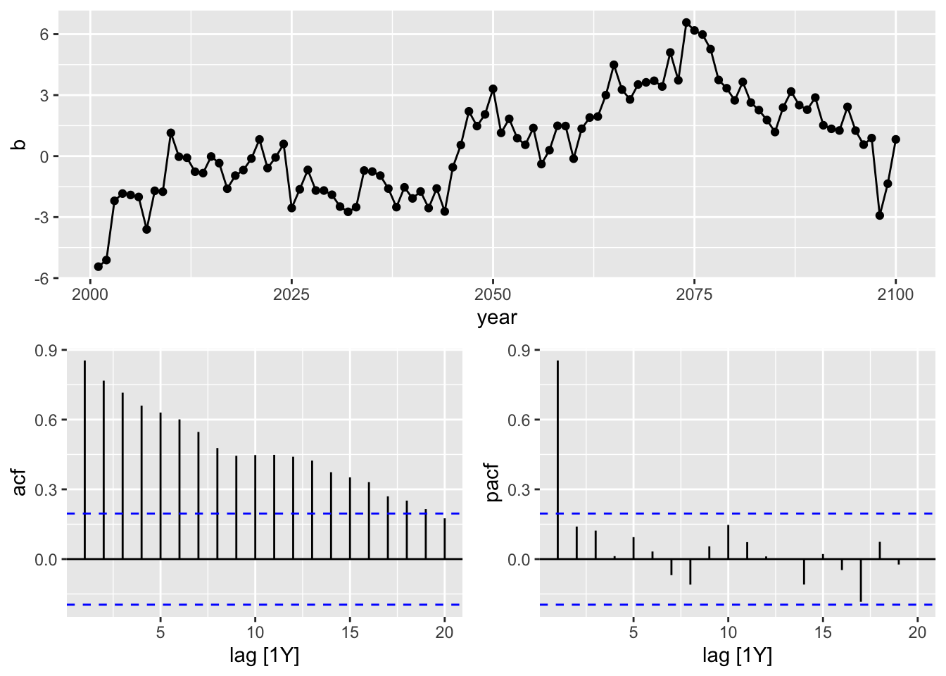
               b = arima.sim(n = 100,
                             model = list(ar = 0.9)),
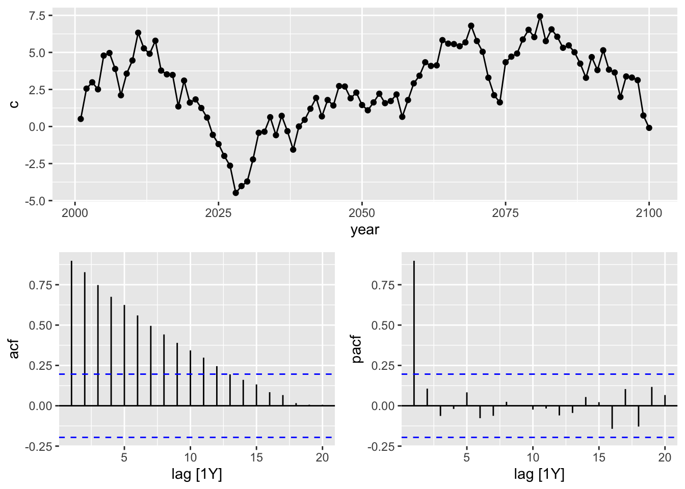
               c = cumsum(rnorm(n = 100, mean = 0, sd = 1)))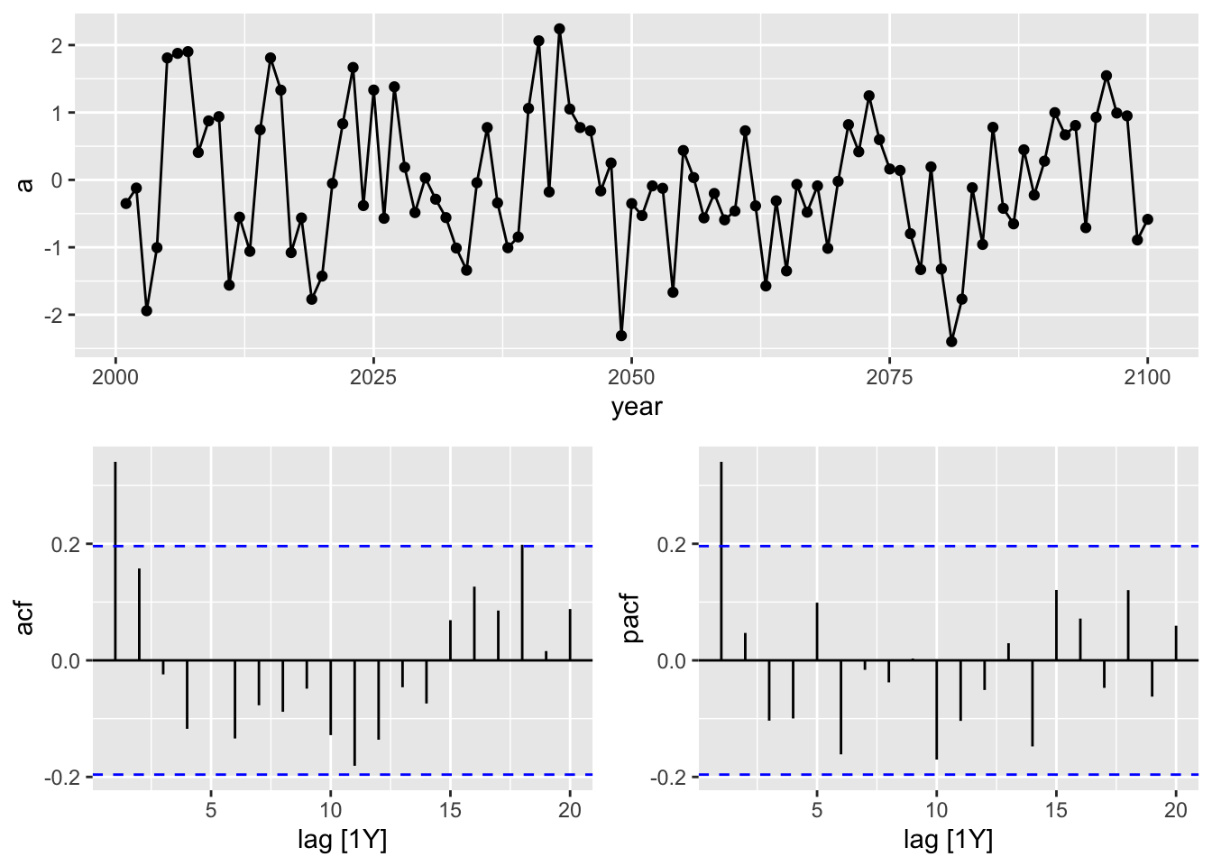

data$year = 2001:2100
data <- data |> as_tsibble(index = year)

data |>
  gg_tsdisplay(a, plot_type = 'partial')

data |>
  gg_tsdisplay(b, plot_type = 'partial')

data |>
  gg_tsdisplay(c, plot_type = 'partial')

train <- data |> filter(year < 2081)

mod_b <- train |>
  model(ar1 = ARIMA(b ~ pdq(1, 0, 0)), # is correct
        ma1 = ARIMA(b ~ pdq(0, 0, 1)),
        naive = NAIVE(b))

mod_c <- train |>
  model(ar1 = ARIMA(c ~ pdq(1, 0, 0)),
        ma1 = ARIMA(c ~ pdq(0, 0, 1)),
        naive = NAIVE(c)) # is correct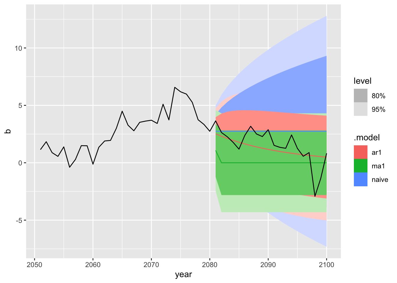

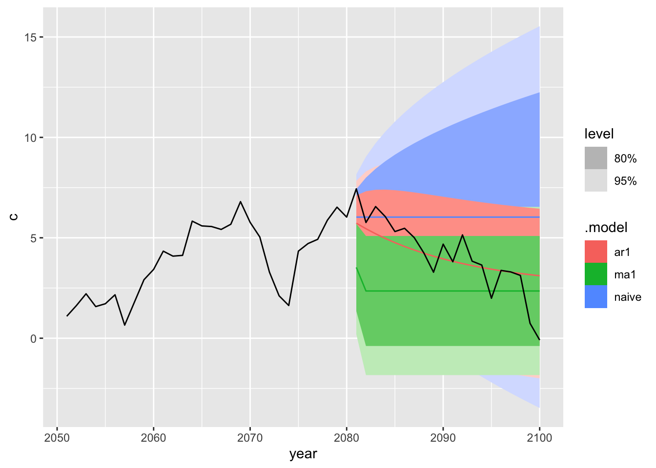
fc_b <- mod_b |> forecast(h = 20)
fc_c <- mod_c |> forecast(h = 20)

fc_b |> autoplot(data |> filter(year > 2050))

fc_c |> autoplot(data |> filter(year > 2050))

5.4 Comparing AR, MA and ARMA

m <- import(paste0(getwd(), '/00_data/marriages.csv'))
glimpse(m)

## Rows: 24,852
## Columns: 4
## $ code  <int64> 1000000000, 1000000000, 1000000000, 1000000000, 1000000000, 1000000000, 1000000000, 1000000000, 1000000000, 1000000000, 1000000000, 1000000000, 1…
## $ name  <chr> "Алтайский край", "Алтайский край", "Алтайский край", "Алтайский край", "Алтайский край", "Алтайский край", "Алтайский край", "Алтайский край", "Ал…
## $ total <int> 953, 1007, 1311, 1554, 562, 1900, 2338, 3034, 2460, 1762, 1411, 1554, 1069, 1221, 1330, 1774, 609, 2107, 2708, 3272, 2483, 1825, 1721, 1940, 1006, …
## $ date  <IDate> 2006-01-01, 2006-02-01, 2006-03-01, 2006-04-01, 2006-05-01, 2006-06-01, 2006-07-01, 2006-08-01, 2006-09-01, 2006-10-01, 2006-11-01, 2006-12-01, 2…

m_agg <- m |> mutate(year = year(date)) |> 
  select(-date) |>
  group_by(code, name, year) |>
  summarise(sum = sum(total),
            max = max(total),
            .groups = 'keep')

glimpse(m_agg)

## Rows: 2,071
## Columns: 5
## Groups: code, name, year [2,071]
## $ code <int64> 30, 30, 30, 30, 30, 30, 30, 30, 30, 30, 30, 30, 30, 30, 30, 30, 30, 30, 30, 31, 31, 31, 31, 31, 31, 31, 31, 31, 31, 31, 31, 31, 31, 31, 31, 31, 31…
## $ name <chr> "Центральный федеральный округ", "Центральный федеральный округ", "Центральный федеральный округ", "Центральный федеральный округ", "Центральный фед…
## $ year <dbl> 2006, 2007, 2008, 2009, 2010, 2011, 2012, 2013, 2014, 2015, 2016, 2017, 2018, 2019, 2020, 2021, 2022, 2023, 2024, 2006, 2007, 2008, 2009, 2010, 2011…
## $ sum  <int> 287557, 328158, 300883, 314089, 311007, 338464, 308879, 317995, 322822, 313157, 263540, 284184, 239977, 259596, 205874, 260025, 295471, 262274, NA, …
## $ max  <int> 40480, 42609, 50269, 45051, 45494, 44597, 44401, 49167, 48272, 44041, 39471, 42925, 41523, 38129, 33330, 37089, 36444, 35476, NA, 14000, 15693, 1800…

rfy <- m_agg |> filter(code == 643) |>
  as_tsibble(index = year)

rfy |>
  gg_tsdisplay(sum, plot_type = 'partial')

## Warning: Removed 1 row containing missing values or values outside the scale range (`geom_line()`).

## Warning: Removed 1 row containing missing values or values outside the scale range (`geom_point()`).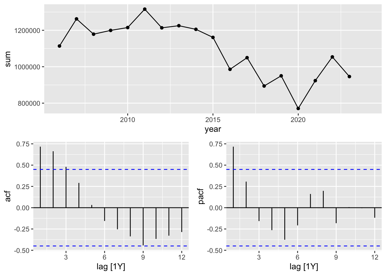

train <- rfy |> filter(year < 2020)

models <- train |>
  model(ar1 = ARIMA(sum ~ pdq(1, 0, 0)),
        ma1 = ARIMA(sum ~ pdq(0, 0, 1)),
        naive = NAIVE(sum),
        arma11 = ARIMA(sum ~ pdq(1, 0, 1)))

report(models$ar1[[1]])

## Series: sum 
## Model: ARIMA(1,0,0) w/ mean 
## 
## Coefficients:
##          ar1   constant
##       0.7069  326218.57
## s.e.  0.1872   20727.82
## 
## sigma^2 estimated as 8.776e+09:  log likelihood=-179.4
## AIC=364.8   AICc=367.2   BIC=366.72

nrow(train)

## [1] 14

nrow(rfy)

## [1] 19

fc <- models |>
  forecast(h = 5)

fc |> accuracy(rfy)

## # A tibble: 4 × 10
##   .model .type       ME    RMSE     MAE    MPE  MAPE  MASE RMSSE    ACF1
##   <chr>  <chr>    <dbl>   <dbl>   <dbl>  <dbl> <dbl> <dbl> <dbl>   <dbl>
## 1 ar1    Test  -115730. 140696. 115730. -13.7  13.7   1.51  1.49 -0.0462
## 2 arma11 Test   -85991. 121657. 102760. -10.5  12.1   1.34  1.29 -0.0138
## 3 ma1    Test  -203169. 221282. 203169. -23.4  23.4   2.64  2.35  0.0541
## 4 naive  Test   -26557. 104471.  78447.  -4.18  9.11  1.02  1.11  0.0716