Chapter 3 ETS model variations

# Libraries loading
library(tidyverse)
library(fpp3)
library(ggplot2)
library(rio)

# data loading
m <- import(paste0(getwd(), '/00_data/marriages.csv'))
glimpse(m)

## Rows: 24,852
## Columns: 4
## $ code  <int64> 1000000000, 1000000000, 1000000000, 1000000000, 1000000000, 1000000000, 1000000000, 1000000000, 1000000000, 1000000000, 1000000000, 1000000000, 1…
## $ name  <chr> "Алтайский край", "Алтайский край", "Алтайский край", "Алтайский край", "Алтайский край", "Алтайский край", "Алтайский край", "Алтайский край", "Ал…
## $ total <int> 953, 1007, 1311, 1554, 562, 1900, 2338, 3034, 2460, 1762, 1411, 1554, 1069, 1221, 1330, 1774, 609, 2107, 2708, 3272, 2483, 1825, 1721, 1940, 1006, …
## $ date  <IDate> 2006-01-01, 2006-02-01, 2006-03-01, 2006-04-01, 2006-05-01, 2006-06-01, 2006-07-01, 2006-08-01, 2006-09-01, 2006-10-01, 2006-11-01, 2006-12-01, 2…

ts_marriages <- m |>
                mutate(date = yearmonth(date)) |>
                as_tsibble(index = date, key = c('code', 'name'))
glimpse(ts_marriages)

## Rows: 24,852
## Columns: 4
## Key: code, name [109]
## $ code  <int64> 30, 30, 30, 30, 30, 30, 30, 30, 30, 30, 30, 30, 30, 30, 30, 30, 30, 30, 30, 30, 30, 30, 30, 30, 30, 30, 30, 30, 30, 30, 30, 30, 30, 30, 30, 30, 3…
## $ name  <chr> "Центральный федеральный округ", "Центральный федеральный округ", "Центральный федеральный округ", "Центральный федеральный округ", "Центральный фе…
## $ total <int> 14845, 16414, 15753, 21803, 9384, 29571, 35691, 39263, 40480, 24137, 21207, 19009, 15433, 17430, 13878, 29703, 10529, 31572, 41328, 42609, 41779, 2…
## $ date  <mth> 2006 Jan, 2006 Feb, 2006 Mar, 2006 Apr, 2006 May, 2006 Jun, 2006 Jul, 2006 Aug, 2006 Sep, 2006 Oct, 2006 Nov, 2006 Dec, 2007 Jan, 2007 Feb, 2007 Ma…

rf_m <- ts_marriages |>
  filter(code == 643, !is.na(total))

3.1 ETS(AAdN): damped trend

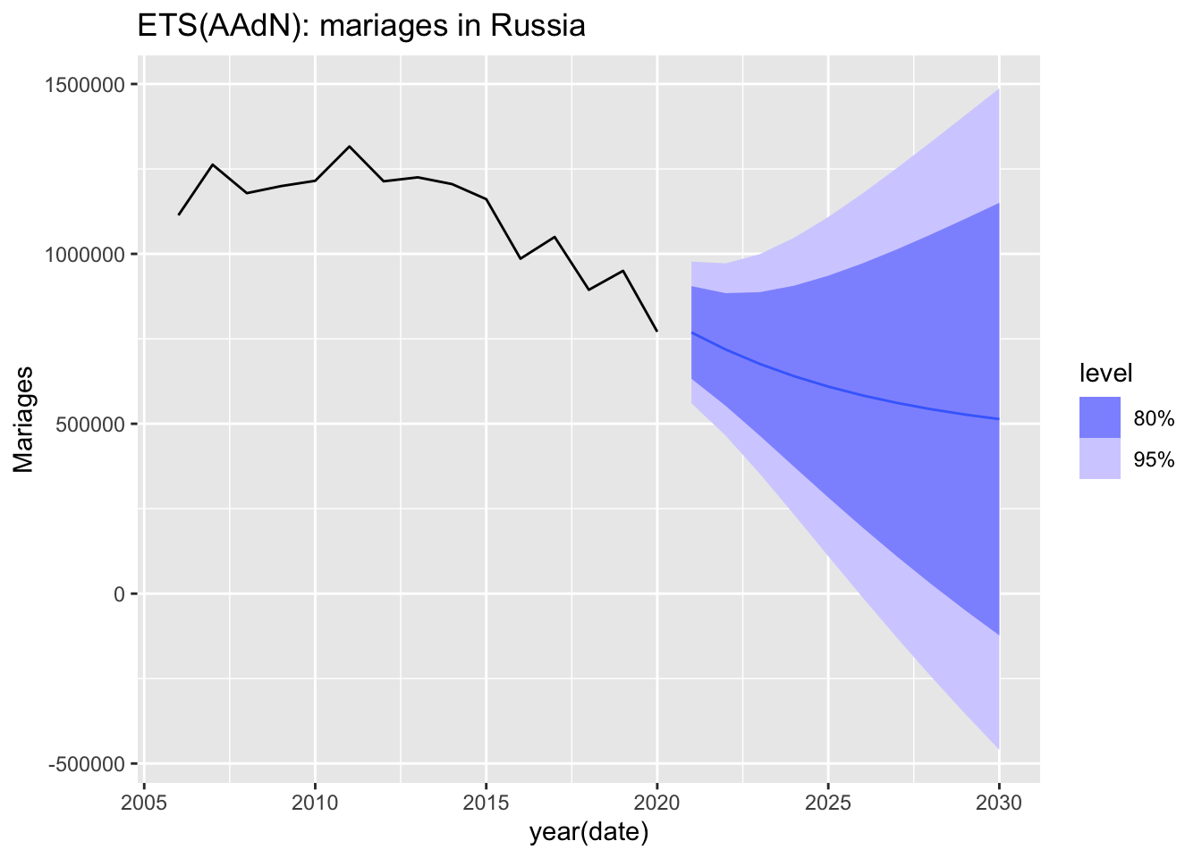
In an ETS model with a damped trend, a special coefficient is added to allow the trend’s growth or decline to slow down over time. This is useful when you expect that the trend will not continue to grow or decrease at the same rate indefinitely but instead will gradually slow down.

A damping parameter \(\phi\) is introduced, which lies between 0 and 1. This parameter controls how the trend slows down. - If \(\phi = 1\), the trend remains additive (linear) and is not damped. - If \(\phi < 1\), the trend gradually reduces, slowing down over time.

In an ETS(AAdN) model (Additive Error, Additive damped Trend, No Seasonality), the model is described as follows:

\[ \begin{cases} y_t = \ell_{t-1} + \phi b _{t-1} + \beta u_t \\ b_t = \phi b _{t-1} + \beta u_t, b_0 - \text {start value} \\ l_t = \ell_{t-1} + \phi b _{t-1} + \alpha u_t, \ell_0 - \text {start value} \\ u_t \sim \mathcal{N}(0,\,\sigma^{2}) \text { and independent} \end{cases} \]

Parameters: \(\alpha, \sigma^2, \ell_0, b_0, \beta, \phi\)

Forecast

One-step forecast

\[ y_{T+1} = \ell_T + \phi b_T + u_{T+1} \]

\[ (y_{T+1}|\mathcal{F_T}) \sim \mathcal{N}(l_T + \phi b_T, \sigma^2) \]

Two-step forecast

\[ y_{T+2} = l_{T+1} + \phi b_{T+1} + u_{T+2} = (l_T + \phi b_T + \alpha u_{T+1}) + \phi(\phi b_T + \beta u_{T+1}) + u_{T+2} \]

\[ (y_{T+2}|\mathcal{F_T}) \sim \mathcal{N}(l_T + (\phi + \phi^2)b_T, \sigma^2((\alpha + \phi \beta)^2 + 1)) \]

Example

rf_y <- rf_m |>
  index_by(year(date)) |>
  summarize(total = sum(total)) |>
  filter(`year(date)` < 2021)

rf_y|>
  model(ETS(total ~ error('A') + trend('Ad') + season('N'))) |>
  forecast(h = 10) |>
  autoplot(rf_y) +
  labs(title = 'ETS(AAdN): mariages in Russia', y = 'Mariages')

3.2 ETS(MNM): multiplicative components

ETS - Error, Trend, Seasonality.
MNM - Multiplicative error, No trend, Mo seasonality.

\[ \begin{cases} y_t = l_{t-1} \times s_{t-12} \times (1 + u_t) \\ l_t = l_{t-1} \times (1 + \alpha u_t), l_0 - \text {start value} \\ s_t = s_{t-12} \times (1 + \gamma u_t), s_0, ..., s_{-11} - \text {start values} \\ u_t \sim \mathcal{N}(0,\,\sigma^{2}) \text { and independent} \end{cases} \]

• \(y_t\) - observed value at time \(t\)
• \(\ell_t\) - trend, or level at time \(T\)
• \(s_t\) - seasonal component
• \(u_t\) - random error

Parameters

• Non-seasonal parameters: \(\alpha, \sigma^2, l_0\)
• Seasonal parameters: \(\gamma, s_0, s_{-1},..., s_{-11}\)

Limitation: \(s_0 \times s_{-1} \times...\times s_{-11} = 1\)

• \(y_t, \ell_t\) - original units
• \(s_t, u_t\) - fraction
• \(s_t\) is measured relative to one, for example, \(s_t = 0.9\) means it is 10% below the trend.
• \(u_t\) is measured relative to zero, for example, \(u_t = -0.1\) means a 10% decrease.

Forecast

One-step forecast

\[ y_{T+1} = l_T \times s_{T-11} \times (1 + u_{T+1}) \]

\[ (y_{T+1}|\mathcal{F_T}) \sim \mathcal{N}(\ell_T \times s_{T-11}, (\ell_T \times s_{T-11})^2\sigma^2) \]

Two-step forecast

\[ y_{T+2} = l_{T+1} \times s_{T-10} \times (1+u_{T+2}) = l_T (1+ \alpha u_{T+1}) \times s_{T-10} \times (1 + u_{T+2}) \]

Example

fc1 <- aus_production |>
  filter(year(Quarter) < 1970) |>
  model(ETS(Electricity ~ error('M') + trend('N') + season('M'))) |>
  forecast(h = 16)

fc2 <- aus_production |>
  filter(year(Quarter) < 1980) |>
  model(ETS(Electricity ~ error('M') + trend('N') + season('M'))) |>
  forecast(h = 16)

aus_production |>
  filter(year(Quarter) < 1980) |>
  autoplot(Electricity) +
  autolayer(fc1) +
  autolayer(fc2) +
  labs(title = 'ETS(MNM): electricity production in Australia')

## Scale for fill_ramp is already present.
## Adding another scale for fill_ramp, which will replace the existing scale.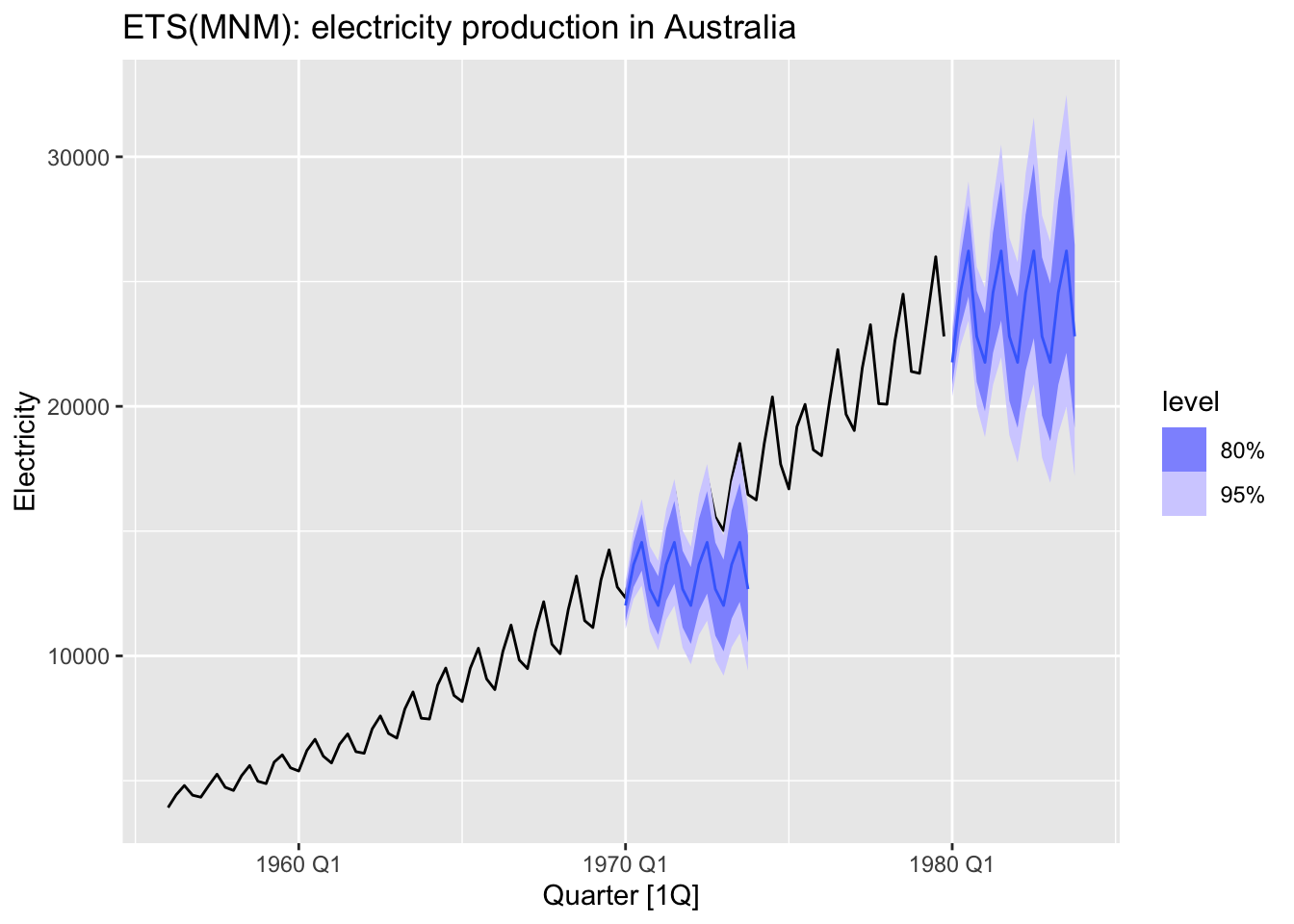

3.3 ETS(MAdM): combinations

MAdM: Multiplicative error, Additive dumped trend, Multiplicative seasonality

\[ \begin{cases} y_t = (l_{t-1} + \phi b_{t-1}) \times s_{t-12} \times (1 + u_t) \\ l_t = (l_{t-1} + \phi b_{t-1}) \times (1 + \alpha u_t), l_0 - \text {start value} \\ b_t = \phi b_{t-1} + \beta(l_{t-1} + \phi b_{t-1})u_t, b_0 - \text {start value}\\ s_t = s_{t-12} \times (1 + \gamma u_t), s_0, ..., s_{-11} - \text {start values} \\ u_t \sim \mathcal{N}(0,\,\sigma^{2}) \text { and independent} \end{cases} \]

Parameters

• Non-seasonal parameters: \(\alpha, \beta, \sigma, \phi, l_0, b_0\)
• Seasonal parameters: \(\gamma, s_0, s_{-1}, ... , s_{-11}\)

Forecast

One-step forecast

\[ y_{T+1} = (l_T + \phi b_T) \times s_{T-11} \times (1 + u_{T+1}) \]

\[ (y_{T+1}|\mathcal{F_T}) \sim \mathcal{N}((\ell_T + \phi b_T) \times s_{T-11}, (\ell_T + \phi b_T)^2 \times s_{T-11}^2 \times \sigma^2) \]

Example

rf_m |>
  filter(year(date) > 2012, year(date) < 2022) |>
  model(ETS(total ~ error('M') + trend('Ad') + season('M'))) |>
  forecast(h = 48) |>
  autoplot(rf_m) +
  labs(title = 'EST(MAdM): forecast')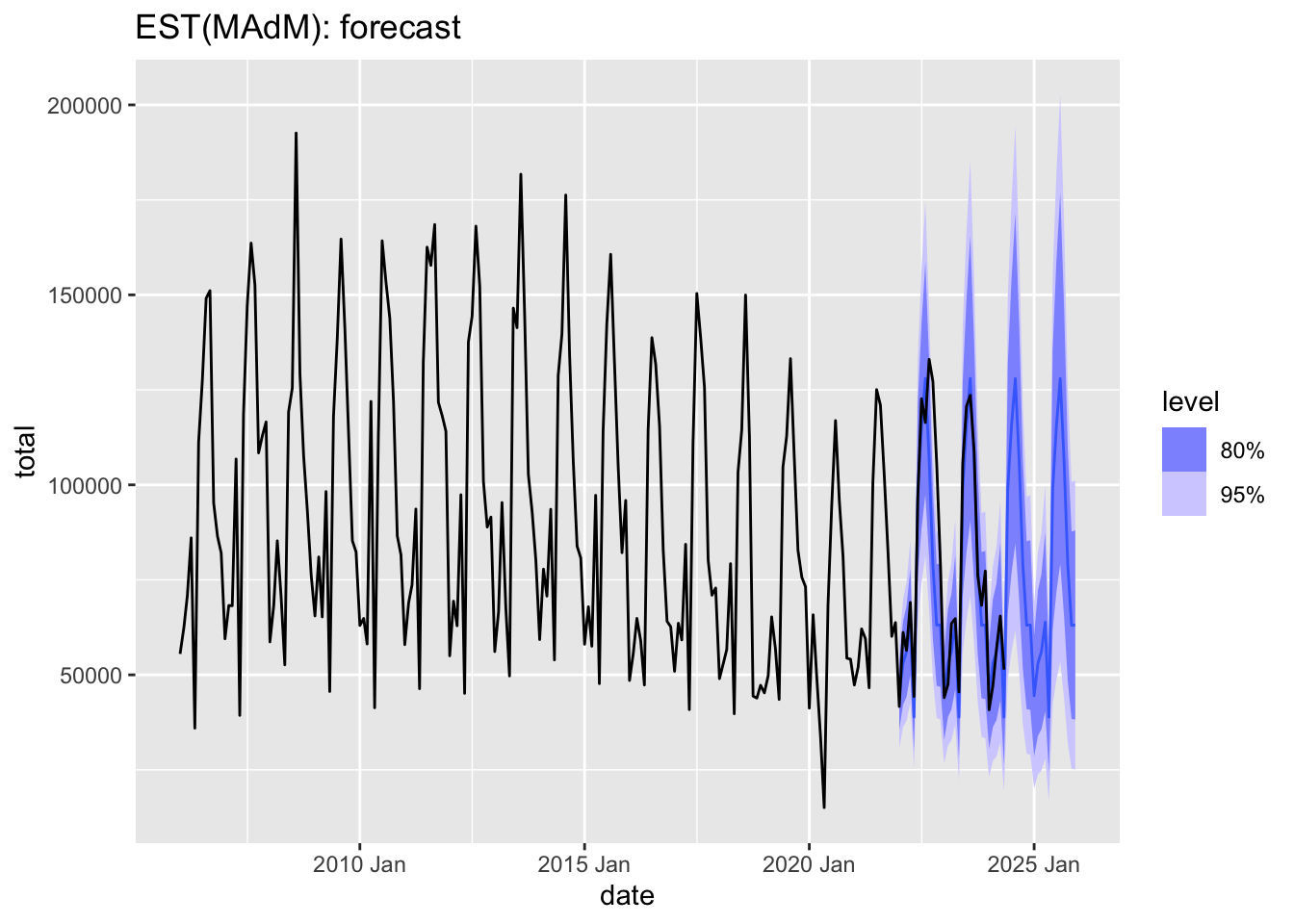

Combinations:

• Errors: A, M
• Trend: N, A, Ad, M, Md
• Seasonality: N, A, M

Historic naming:

• ETS(ANN) - Simple Exponential Smoothing
• ETS(AAA) - Additive Holt-Winters Method
• ETS(AAM) - Multiplicative Holt-Winters Method
• ETS(AAdM) - Damped Additive Trend with Multiplicative Seasonality (Damped Holt-Winters)

3.4 Examples

rf_m |>
  gg_tsdisplay(total)

Split into training and test set.

rf_train <- rf_m |>
      filter(year(date) < 2020)
rf_test <- rf_m |>
  anti_join(rf_train, by = 'date')

models <- rf_train |>
  model(
    snaive = SNAIVE(total),
    ANA = ETS(total ~ error('A') + trend('N') + season('A')),
    AAA = ETS(total ~ error('A') + trend('A') + season('A')),
    AAdA = ETS(total ~ error('A') + trend('Ad') + season('A')),
    zzz = ETS(total), # select the best model by AIC
    azz = ETS(total ~ error('A')),
    theta = THETA(total) # theta method
  )

models$zzz[[1]] |> report()

## Series: total 
## Model: ETS(M,N,M) 
##   Smoothing parameters:
##     alpha = 0.09614705 
##     gamma = 0.0001025139 
## 
##   Initial states:
##      l[0]      s[0]    s[-1]    s[-2]    s[-3]    s[-4]    s[-5]    s[-6]     s[-7]     s[-8]    s[-9]    s[-10]    s[-11]
##  98845.29 0.8608546 0.876489 1.033511 1.431267 1.673549 1.454279 1.274721 0.4759065 0.9107223 0.736584 0.6824381 0.5896779
## 
##   sigma^2:  0.017
## 
##      AIC     AICc      BIC 
## 4023.088 4026.246 4069.947

models$theta[[1]] |> report()

## Series: total 
## Model: THETA 
## 
## Alpha: 0.1385 
## Drift: -71.6835 
## sigma^2: 141532473.0062

fc <- models |>
  forecast(h = 72)

fc |> accuracy(rf_m)

## Warning: The future dataset is incomplete, incomplete out-of-sample data will be treated as missing. 
## 19 observations are missing between 2024 Jun and 2025 Dec

## # A tibble: 7 × 12
##   .model    code name                 .type      ME   RMSE    MAE    MPE  MAPE  MASE RMSSE  ACF1
##   <chr>  <int64> <chr>                <chr>   <dbl>  <dbl>  <dbl>  <dbl> <dbl> <dbl> <dbl> <dbl>
## 1 AAA        643 Российская Федерация Test   9524.  20089. 16578. 14.3    26.1 1.37  1.25  0.534
## 2 AAdA       643 Российская Федерация Test   2156.  16373. 12366.  3.07   19.2 1.02  1.02  0.458
## 3 ANA        643 Российская Федерация Test    -57.3 16139. 11922. -0.401  18.4 0.987 1.01  0.452
## 4 azz        643 Российская Федерация Test    -57.3 16139. 11922. -0.401  18.4 0.987 1.01  0.452
## 5 snaive     643 Российская Федерация Test  -1987.  14026. 10311. -7.60   17.0 0.853 0.874 0.470
## 6 theta      643 Российская Федерация Test    115.  14283. 10025. -4.25   16.5 0.830 0.890 0.545
## 7 zzz        643 Российская Федерация Test  -1830.  14036. 10206. -6.92   16.9 0.845 0.874 0.500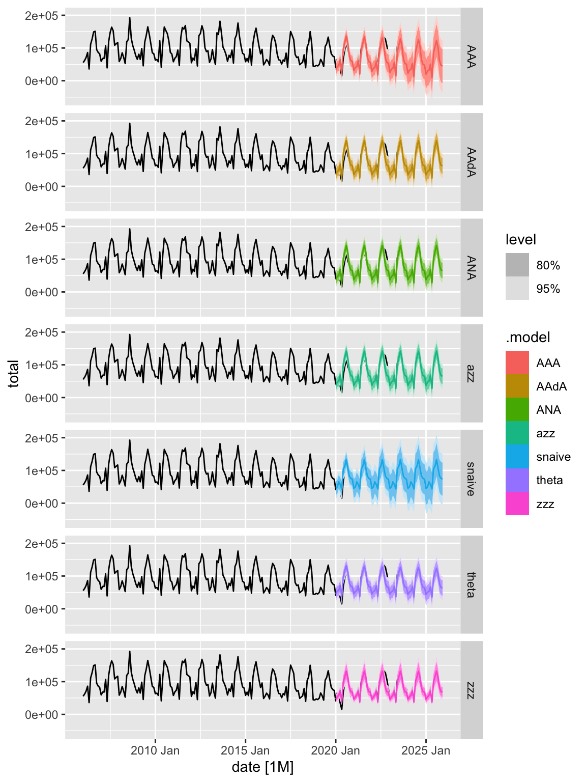

rf_m |>
  autoplot(total) +
  autolayer(fc) +
  facet_grid(.model ~ .)

Composite model.

models <- rf_train |>
  model(
    snaive = SNAIVE(total),
    theta = THETA(total),
    composit = decomposition_model(
      STL(total ~ season(window = Inf)),
      ETS(season_adjust ~ error('A') + trend('Ad') + season('N')),
      SNAIVE(season_year) ))

models |>
  forecast(h = 48) |>
  accuracy(rf_m)

## # A tibble: 3 × 12
##   .model      code name                 .type      ME   RMSE    MAE   MPE  MAPE  MASE RMSSE  ACF1
##   <chr>    <int64> <chr>                <chr>   <dbl>  <dbl>  <dbl> <dbl> <dbl> <dbl> <dbl> <dbl>
## 1 composit     643 Российская Федерация Test   3863.  17186. 13390.  4.97  20.4 1.11  1.07  0.490
## 2 snaive       643 Российская Федерация Test  -2213.  14571. 10717. -8.33  17.6 0.887 0.908 0.479
## 3 theta        643 Российская Федерация Test    -42.7 14814. 10474. -4.98  17.0 0.867 0.923 0.567

Model evaluation for multiple time series.

train <- ts_marriages |>
  filter(year(date) < 2020)

models <- train |>
  model(
    snaive = SNAIVE(total),
    zzz = ETS(log(total)), # select the best model by AIC
    theta = THETA(total)
  )

## Warning: 22 errors (2 unique) encountered for zzz
## [21] ETS does not support missing values.
## [1] NA/NaN/Inf in 'y'

## Warning: 21 errors (1 unique) encountered for theta
## [21] missing values in object

acc <- models |>
  forecast(h = 48) |> 
  accuracy(rf_m)

## Warning: The future dataset is incomplete, incomplete out-of-sample data will be treated as missing. 
## 48 observations are missing between 2020 Jan and 2023 Dec

acc |>
  group_by(.model) |>
  summarise(avg_MAE = mean(MAE, na.rm = TRUE))

## # A tibble: 3 × 2
##   .model avg_MAE
##   <chr>    <dbl>
## 1 snaive  74637.
## 2 theta   74759.
## 3 zzz     74672.