Chapter 10 Dynamic regression models

The source of the chapter

# loading libraries
library(tsibble)
library(tsibbledata)
library(tidyverse)
# to read data
library(rio)
library(ggplot2)
library(fabletools)
library(feasts)
library(fpp3)
library(latex2exp)
library(forecast)

10.1 Regression with ARIMA errors using fable

The source of the section

To fit a regression model with ARIMA errors, the pdq() specifies the order of the ARIMA errors model.

If differencing is specifies, then the differencing is applied to all variables in the regression model. Use ARIMA(y ~ x + pdq(1,1,0)) to apply dirfferencing to all variables.

The constant disappears due to the differencing. Add 1 to include the constant.

10.1.1 Example: US Personal Consumption and Income

us_change |>
  pivot_longer(c(Consumption, Income),
               names_to = 'var', values_to = 'value') |>
  autoplot(value) +
  facet_grid(var ~ ., scales = 'free_y') +
  labs(title = "US consumption and personal income",
       y = "Quarterly % change") +
    theme(legend.position ='none')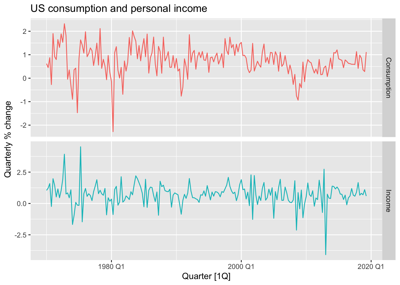

fit <- us_change |>
  model(ARIMA(Consumption ~ Income))

fit |> report()

## Series: Consumption 
## Model: LM w/ ARIMA(1,0,2) errors 
## 
## Coefficients:
##          ar1      ma1     ma2  Income  intercept
##       0.7070  -0.6172  0.2066  0.1976     0.5949
## s.e.  0.1068   0.1218  0.0741  0.0462     0.0850
## 
## sigma^2 estimated as 0.3113:  log likelihood=-163.04
## AIC=338.07   AICc=338.51   BIC=357.8

bind_rows(
    `Regression residuals` =
        as_tibble(residuals(fit, type = "regression")),
    `ARIMA residuals` =
        as_tibble(residuals(fit, type = "innovation")),
    .id = "type"
  ) |>
  mutate(
    type = factor(type, levels=c(
      "Regression residuals", "ARIMA residuals"))
  ) |>
  ggplot(aes(x = Quarter, y = .resid)) +
  geom_line() +
  facet_grid(vars(type))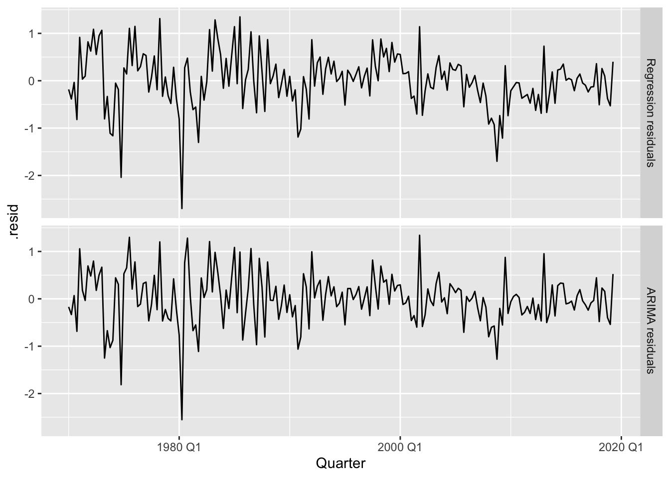

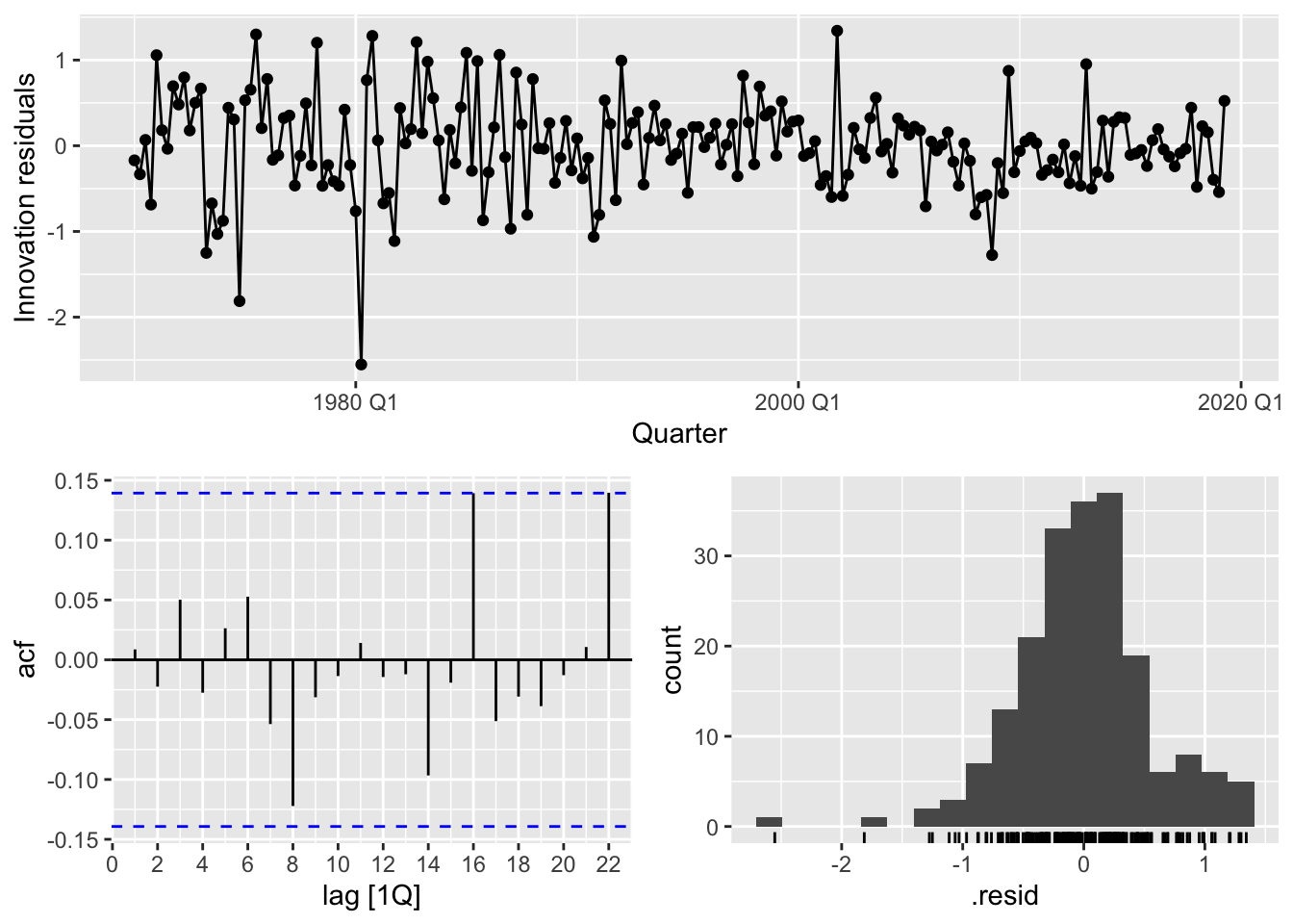
fit |> gg_tsresiduals()

augment(fit) |>
  features(.innov, ljung_box, dof = 3, lag = 8)

## # A tibble: 1 × 3
##   .model                      lb_stat lb_pvalue
##   <chr>                         <dbl>     <dbl>
## 1 ARIMA(Consumption ~ Income)    5.21     0.391

We cannot reject \(H_0\), so there is no autocorrelation in the residuals.

10.2 Forecasting

The source of the section

To forecast using a regression model with ARIMA errors, we need to forecast the regression part of the model and the ARIMA part of the model, and combine the results. When the predictors are themselves unknown, we must either model them separately, or use assumed future values for each predictor.

10.2.1 Example: US Personal Consumption and Income

us_change_future <- new_data(us_change, 8) |>
  mutate(Income = mean(us_change$Income))

fit |> 
  forecast(new_data = us_change_future) |>
  autoplot(us_change) +
  labs(y = "Percentage change")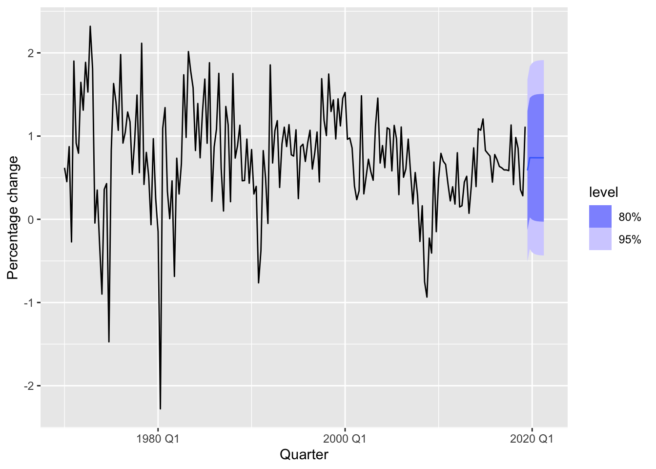

10.2.2 Example: Forecasting electricity demand

vic_elec_daily <- vic_elec |>
  filter(year(Time) == 2014) |>
  index_by(Date = date(Time)) |>
  summarise(
    Demand = sum(Demand) / 1e3,
    Temperature = max(Temperature),
    Holiday = any(Holiday)
  ) |>
  mutate(Day_Type = case_when(
    Holiday ~ "Holiday",
    wday(Date) %in% 2:6 ~ "Weekday",
    TRUE ~ "Weekend"
  ))

vic_elec_daily |>
  ggplot(aes(x = Temperature, y = Demand, colour = Day_Type)) +
  geom_point() +
  labs(y = "Electricity demand (GW)",
       x = "Maximum daily temperature")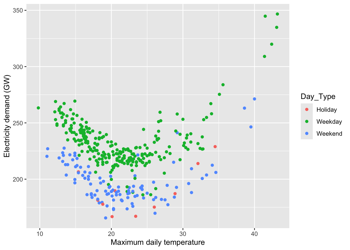

vic_elec_daily |>
  pivot_longer(c(Demand, Temperature)) |>
  ggplot(aes(x = Date, y = value)) +
  geom_line() +
  facet_grid(name ~ ., scales = "free_y") + ylab("")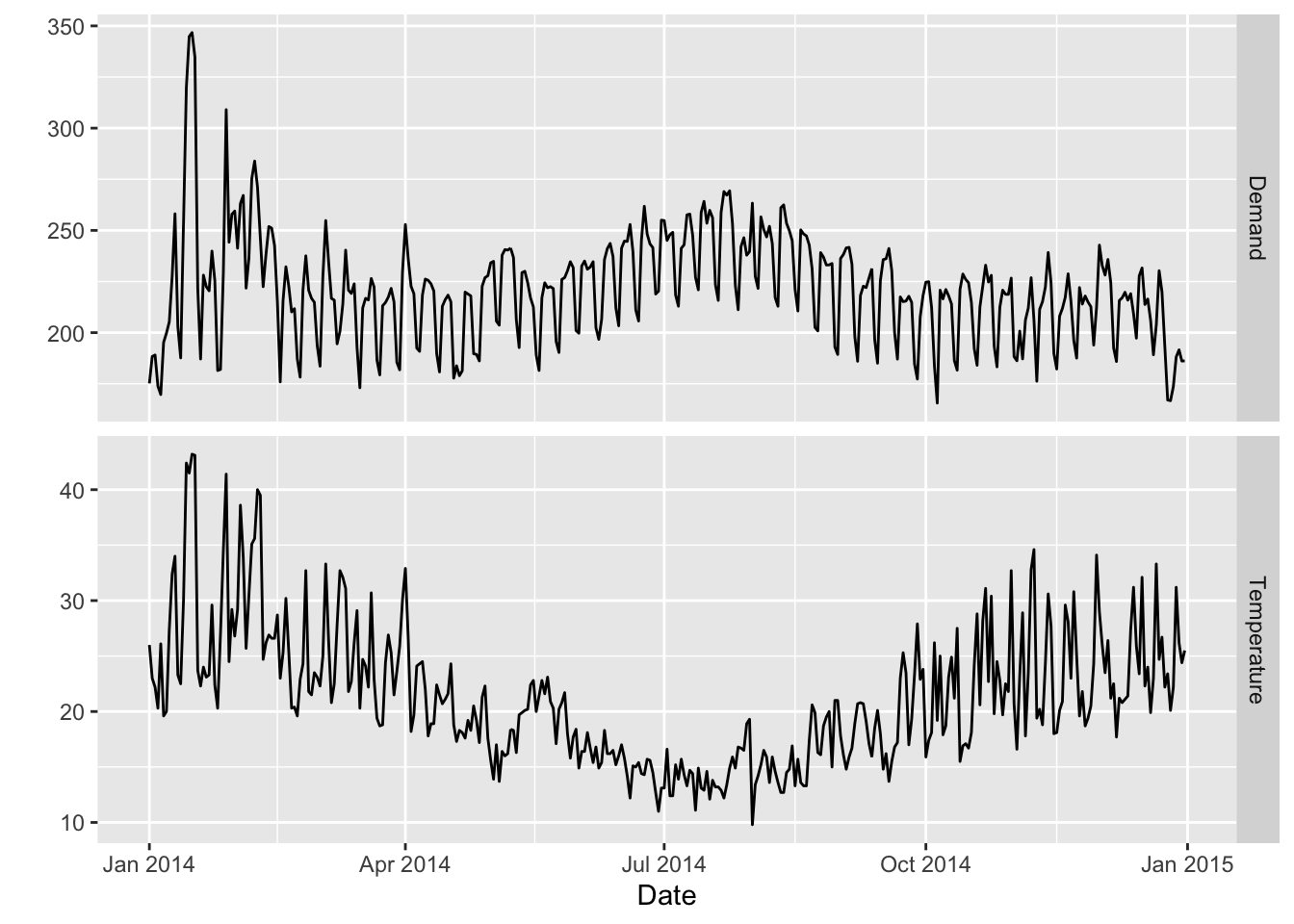

fit <- vic_elec_daily |>
  model(ARIMA(Demand ~ Temperature + I(Temperature^2) +
                (Day_Type == "Weekday")))
fit |> gg_tsresiduals()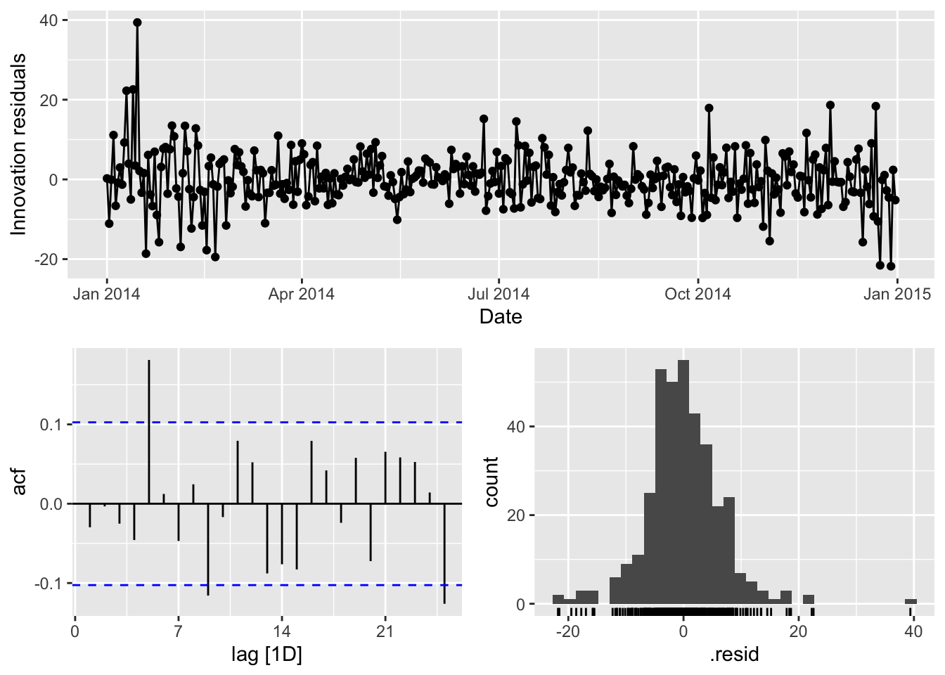

# dof = p + q + P + Q = 2 + 2 + 2 + 0

augment(fit) |>
  features(.innov, ljung_box, dof = 6, lag = 14)

## # A tibble: 1 × 3
##   .model                                                                             lb_stat lb_pvalue
##   <chr>                                                                                <dbl>     <dbl>
## 1 "ARIMA(Demand ~ Temperature + I(Temperature^2) + (Day_Type == \n    \"Weekday\"))"    28.4  0.000404

vic_elec_future <- new_data(vic_elec_daily, 14) |>
  mutate(
    Temperature = 26,
    Holiday = c(TRUE, rep(FALSE, 13)),
    Day_Type = case_when(
      Holiday ~ "Holiday",
      wday(Date) %in% 2:6 ~ "Weekday",
      TRUE ~ "Weekend"
    )
  )
forecast(fit, vic_elec_future) |>
  autoplot(vic_elec_daily) +
  labs(title="Daily electricity demand: Victoria",
       y="GW")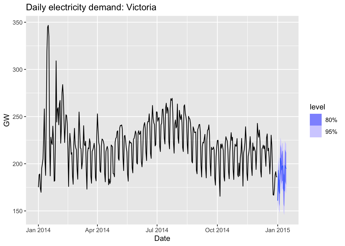

10.3 Stochastic and deterministic trends

The source of the section

10.3.1 Example: Air transport passengers Australia

aus_airpassengers |>
  autoplot(Passengers) +
  labs(y = 'Passengers (millions)',
       title = 'Total annual air passengers')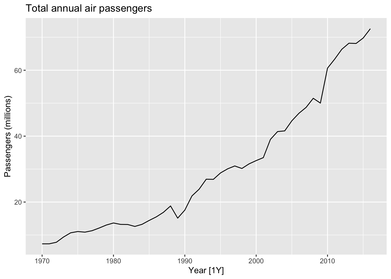

1. The deterministic trend model

fit_deterministic <- aus_airpassengers |>
  model(deterministic = ARIMA(Passengers ~ 1 + trend() + pdq(d = 0)))

fit_deterministic |> report()

## Series: Passengers 
## Model: LM w/ ARIMA(1,0,0) errors 
## 
## Coefficients:
##          ar1  trend()  intercept
##       0.9564   1.4151     0.9014
## s.e.  0.0362   0.1972     7.0751
## 
## sigma^2 estimated as 4.343:  log likelihood=-100.88
## AIC=209.77   AICc=210.72   BIC=217.17

2. The stochastic trend model

fit_stochastic <- aus_airpassengers |>
  model(stochastic = ARIMA(Passengers ~ pdq(d = 1)))

fit_stochastic |> report()

## Series: Passengers 
## Model: ARIMA(0,1,0) w/ drift 
## 
## Coefficients:
##       constant
##         1.4191
## s.e.    0.3014
## 
## sigma^2 estimated as 4.271:  log likelihood=-98.16
## AIC=200.31   AICc=200.59   BIC=203.97

aus_airpassengers |>
  autoplot(Passengers) +
  autolayer(fit_stochastic |> forecast(h = 20),
    colour = "#0072B2", level = 95) +
  autolayer(fit_deterministic |> forecast(h = 20),
    colour = "#D55E00", alpha = 0.65, level = 95) +
  labs(y = "Air passengers (millions)",
       title = "Forecasts from trend models")

## Scale for fill_ramp is already present.
## Adding another scale for fill_ramp, which will replace the existing scale.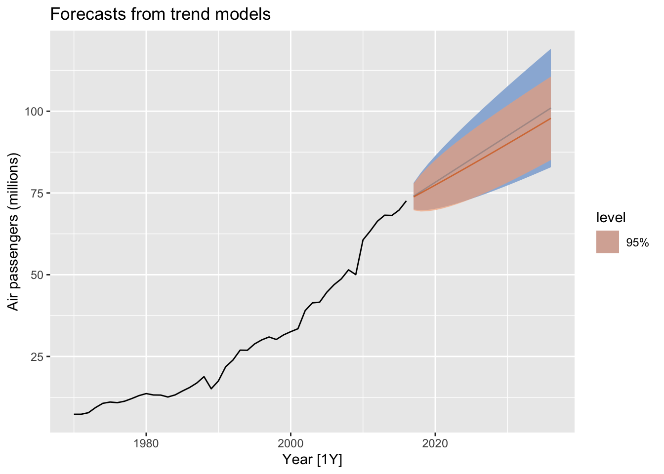

• The slope of the deterministic trend is not going to change over time.
• It is safer to forecast with stochastic trends, especially for longer forecast horizons, as the prediction intervals allow for greater uncertainty in future growth.

10.4 Dynamic harmonic regression

The source of the section

The dynamic regression with Fourier terms is often better for long seasonal periods.

The ARIMA() function is allow a seasonal period up to \(m=350\).

The harmonic regression allows:

• any length seasonality
• Fourier terms of different frequencies can be used for data with more than one seasonal period
• \(K\) param controls the smoothness of the seasonal pattern. It is the number of Fourier sin and cos pairs. The smaller \(K\) is, the smoother the seasonal pattern is.

The seasonality has to have fixed pattern over time.

10.5 Example: Australian eating out expenditure

aus_cafe <- aus_retail |>
  filter(
    Industry == "Cafes, restaurants and takeaway food services",
    year(Month) %in% 2004:2018
  ) |>
  summarise(Turnover = sum(Turnover))

fit <- model(aus_cafe,
  `K = 1` = ARIMA(log(Turnover) ~ fourier(K=1) + PDQ(0,0,0)),
  `K = 2` = ARIMA(log(Turnover) ~ fourier(K=2) + PDQ(0,0,0)),
  `K = 3` = ARIMA(log(Turnover) ~ fourier(K=3) + PDQ(0,0,0)),
  `K = 4` = ARIMA(log(Turnover) ~ fourier(K=4) + PDQ(0,0,0)),
  `K = 5` = ARIMA(log(Turnover) ~ fourier(K=5) + PDQ(0,0,0)),
  `K = 6` = ARIMA(log(Turnover) ~ fourier(K=6) + PDQ(0,0,0)),
)

fit |>
  forecast(h = "2 years") |>
  autoplot(aus_cafe, level = 95) +
  facet_wrap(vars(.model), ncol = 2) +
  guides(colour = "none", fill = "none", level = "none") +
  geom_label(
    aes(x = yearmonth("2007 Jan"), y = 4250,
        label = paste0("AICc = ", format(AICc))),
    data = glance(fit)
  ) +
  labs(title= "Total monthly eating-out expenditure",
       y="$ billions")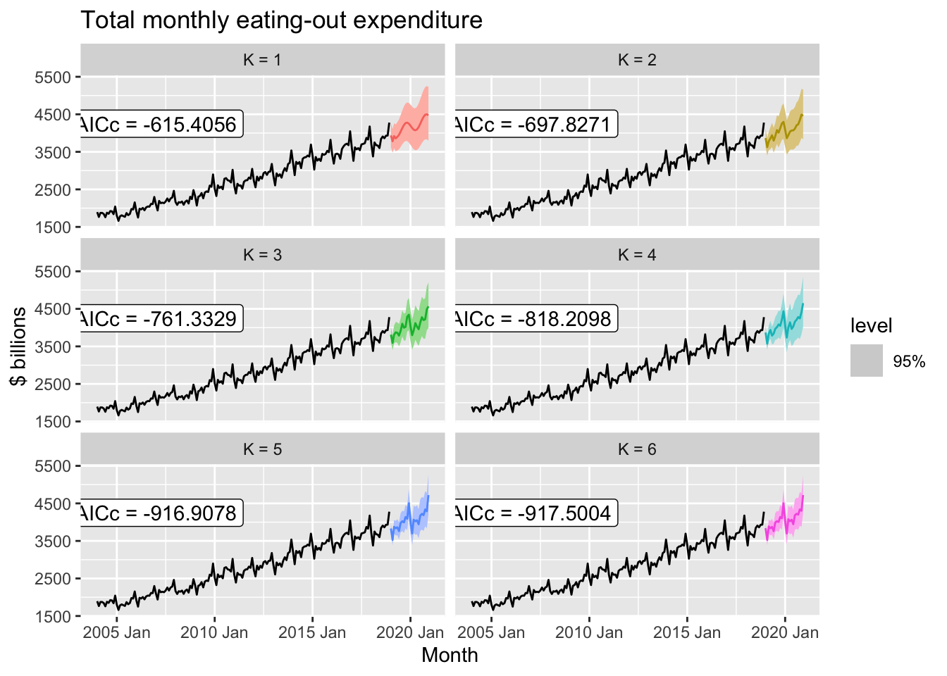

10.6 Lagged predictors

The source of the section

10.6.1 Example: TV advertising and insurance quotations

insurance |>
  pivot_longer(Quotes:TVadverts) |>
  ggplot(aes(x = Month, y = value)) +
  geom_line() +
  facet_grid(vars(name), scales = "free_y") +
  labs(y = "", title = "Insurance advertising and quotations")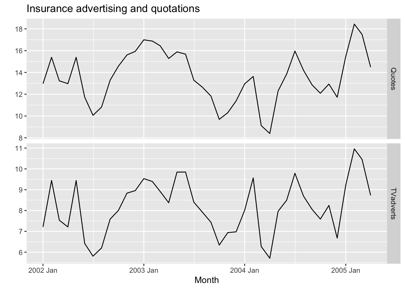

fit <- insurance |>
  # Restrict data so models use same fitting period
  mutate(Quotes = c(NA, NA, NA, Quotes[4:40])) |>
  # Estimate models
  model(
    lag0 = ARIMA(Quotes ~ pdq(d = 0) + TVadverts),
    lag1 = ARIMA(Quotes ~ pdq(d = 0) +
                 TVadverts + lag(TVadverts)),
    lag2 = ARIMA(Quotes ~ pdq(d = 0) +
                 TVadverts + lag(TVadverts) +
                 lag(TVadverts, 2)),
    lag3 = ARIMA(Quotes ~ pdq(d = 0) +
                 TVadverts + lag(TVadverts) +
                 lag(TVadverts, 2) + lag(TVadverts, 3))
  )

fit |> glance()

## # A tibble: 4 × 8
##   .model sigma2 log_lik   AIC  AICc   BIC ar_roots  ma_roots 
##   <chr>   <dbl>   <dbl> <dbl> <dbl> <dbl> <list>    <list>   
## 1 lag0    0.265   -28.3  66.6  68.3  75.0 <cpl [2]> <cpl [0]>
## 2 lag1    0.209   -24.0  58.1  59.9  66.5 <cpl [1]> <cpl [1]>
## 3 lag2    0.215   -24.0  60.0  62.6  70.2 <cpl [1]> <cpl [1]>
## 4 lag3    0.206   -22.2  60.3  65.0  73.8 <cpl [1]> <cpl [1]>

fit_best <- insurance |>
  model(ARIMA(Quotes ~ pdq(d = 0) +
              TVadverts + lag(TVadverts)))
report(fit_best)

## Series: Quotes 
## Model: LM w/ ARIMA(1,0,2) errors 
## 
## Coefficients:
##          ar1     ma1     ma2  TVadverts  lag(TVadverts)  intercept
##       0.5123  0.9169  0.4591     1.2527          0.1464     2.1554
## s.e.  0.1849  0.2051  0.1895     0.0588          0.0531     0.8595
## 
## sigma^2 estimated as 0.2166:  log likelihood=-23.94
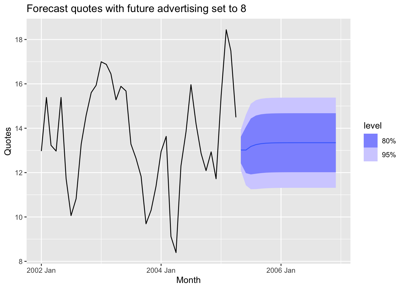
## AIC=61.88   AICc=65.38   BIC=73.7

insurance_future <- new_data(insurance, 20) |>
  mutate(TVadverts = 8)
fit_best |>
  forecast(insurance_future) |>
  autoplot(insurance) +
  labs(
    y = "Quotes",
    title = "Forecast quotes with future advertising set to 8"
  )