Chapter 4 Time series features
# loading libraries
library(tsibble)
library(tsibbledata)
library(tidyverse)
# to read data
library(rio)
library(ggplot2)
library(fabletools)
library(feasts)
library(fpp3)
library(latex2exp)
library(forecast)
Different features of time series could be used to explore the properties of the series.
4.1 Some simple statistics
## # A tibble: 304 × 4
##    Region          State Purpose   mean
##    <chr>           <chr> <chr>    <dbl>
##  1 Kangaroo Island SA    Other    0.340
##  2 MacDonnell      NT    Other    0.449
##  3 Wilderness West TAS   Other    0.478
##  4 Barkly          NT    Other    0.632
##  5 Clare Valley    SA    Other    0.898
##  6 Barossa         SA    Other    1.02
##  7 Kakadu Arnhem   NT    Other    1.04
##  8 Lasseter        NT    Other    1.14
##  9 Wimmera         VIC   Other    1.15
## 10 MacDonnell      NT    Visiting 1.18
## # ℹ 294 more rows## # A tibble: 304 × 8
## Region State Purpose `0%` `25%` `50%` `75%` `100%`
## <chr> <chr> <chr> <dbl> <dbl> <dbl> <dbl> <dbl>
## 1 Adelaide SA Business 68.7 134. 153. 177. 242.
## 2 Adelaide SA Holiday 108. 135. 154. 172. 224.
## 3 Adelaide SA Other 25.9 43.9 53.8 62.5 107.
## 4 Adelaide SA Visiting 137. 179. 206. 229. 270.
## 5 Adelaide Hills SA Business 0 0 1.26 3.92 28.6
## 6 Adelaide Hills SA Holiday 0 5.77 8.52 14.1 35.8
## 7 Adelaide Hills SA Other 0 0 0.908 2.09 8.95
## 8 Adelaide Hills SA Visiting 0.778 8.91 12.2 16.8 81.1
## 9 Alice Springs NT Business 1.01 9.13 13.3 18.5 34.1
## 10 Alice Springs NT Holiday 2.81 16.9 31.5 44.8 76.5
## # ℹ 294 more rows4.1.1 ACF features
## # A tibble: 304 × 10
##    Region         State Purpose      acf1 acf10 diff1_acf1 diff1_acf10 diff2_acf1 diff2_acf10 season_acf1
##    <chr>          <chr> <chr>       <dbl> <dbl>      <dbl>       <dbl>      <dbl>       <dbl>       <dbl>
##  1 Adelaide       SA    Business  0.0333  0.131     -0.520       0.463     -0.676       0.741      0.201
##  2 Adelaide       SA    Holiday   0.0456  0.372     -0.343       0.614     -0.487       0.558      0.351
##  3 Adelaide       SA    Other     0.517   1.15      -0.409       0.383     -0.675       0.792      0.342
##  4 Adelaide       SA    Visiting  0.0684  0.294     -0.394       0.452     -0.518       0.447      0.345
##  5 Adelaide Hills SA    Business  0.0709  0.134     -0.580       0.415     -0.750       0.746     -0.0628
##  6 Adelaide Hills SA    Holiday   0.131   0.313     -0.536       0.500     -0.716       0.906      0.208
##  7 Adelaide Hills SA    Other     0.261   0.330     -0.253       0.317     -0.457       0.392      0.0745
##  8 Adelaide Hills SA    Visiting  0.139   0.117     -0.472       0.239     -0.626       0.408      0.170
##  9 Alice Springs  NT    Business  0.217   0.367     -0.500       0.381     -0.658       0.587      0.315
## 10 Alice Springs  NT    Holiday  -0.00660 2.11      -0.153       2.11      -0.274       1.55       0.729
## # ℹ 294 more rows
4.1.2 STL features
- Strength of trend:
For strongly trended data, the seasonally adjusted data should have much more variation than the remainder But for data with little or no trend, the two variances should be approximately the same.
\[ F_T = max(0, 1 - \frac {Var(R_t)} {Var(T_t + R_t)}), [0, 1] \]
- Strength of seasonality:
A series with seasonal strength \(F_S\) close to 0 exhibits almost no seasonality, while a series with strong seasonality will have \(F_S\) close to 1.
\[ F_S = max(0, 1 - \frac {Var(R_t)} {Var(S_t + R_t)}), [0, 1] \]
## # A tibble: 304 × 12
## Region State Purpose trend_strength seasonal_strength_year seasonal_peak_year seasonal_trough_year spikiness linearity curvature stl_e_acf1 stl_e_acf10
## <chr> <chr> <chr> <dbl> <dbl> <dbl> <dbl> <dbl> <dbl> <dbl> <dbl> <dbl>
## 1 Adelaide SA Business 0.464 0.407 3 1 158. -5.31 71.6 -0.532 0.594
## 2 Adelaide SA Holiday 0.554 0.619 1 2 9.17 49.0 78.7 -0.510 0.561
## 3 Adelaide SA Other 0.746 0.202 2 1 2.10 95.1 43.4 -0.351 0.403
## 4 Adelaide SA Visiting 0.435 0.452 1 3 56.1 34.6 71.4 -0.501 1.01
## 5 Adelaide Hills SA Business 0.464 0.179 3 0 0.103 0.968 -3.22 -0.600 0.497
## 6 Adelaide Hills SA Holiday 0.528 0.296 2 1 0.177 10.5 24.0 -0.481 0.350
## 7 Adelaide Hills SA Other 0.593 0.404 2 2 0.000444 4.28 3.19 -0.298 0.281
## 8 Adelaide Hills SA Visiting 0.488 0.254 0 3 6.50 34.2 -0.529 -0.472 0.446
## 9 Alice Springs NT Business 0.534 0.251 0 1 0.169 23.8 19.5 -0.492 0.548
## 10 Alice Springs NT Holiday 0.381 0.832 3 1 0.739 -19.6 10.5 -0.522 0.726
## # ℹ 294 more rowsTo identify what type of series are heavily trended and what are most seasonal.
tourism |>
features(Trips, feat_stl) |>
ggplot(aes(x = trend_strength, y = seasonal_strength_year, col = Purpose)) +
geom_point() +
facet_wrap(vars(State))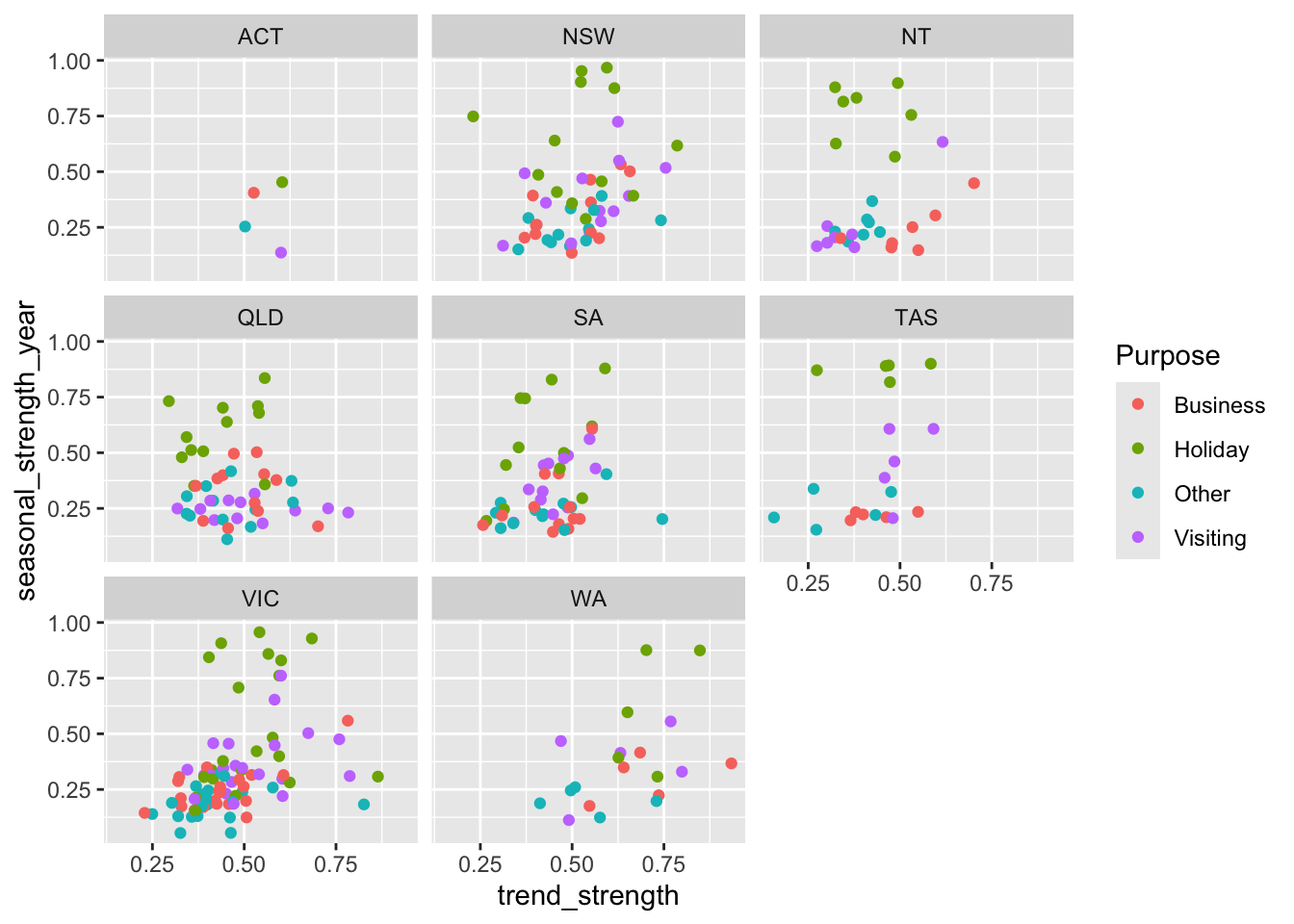
The most seasonal series can also be easily identified and plotted.
tourism |>
  features(Trips, feat_stl) |>
  filter(seasonal_strength_year == max(seasonal_strength_year)) |>
  left_join(tourism, by=c('State', 'Region', 'Purpose'), multiple='all') |>
  ggplot(aes(x = Quarter, y = Trips)) +
  geom_line() +
  facet_wrap(vars(State, Region, Purpose))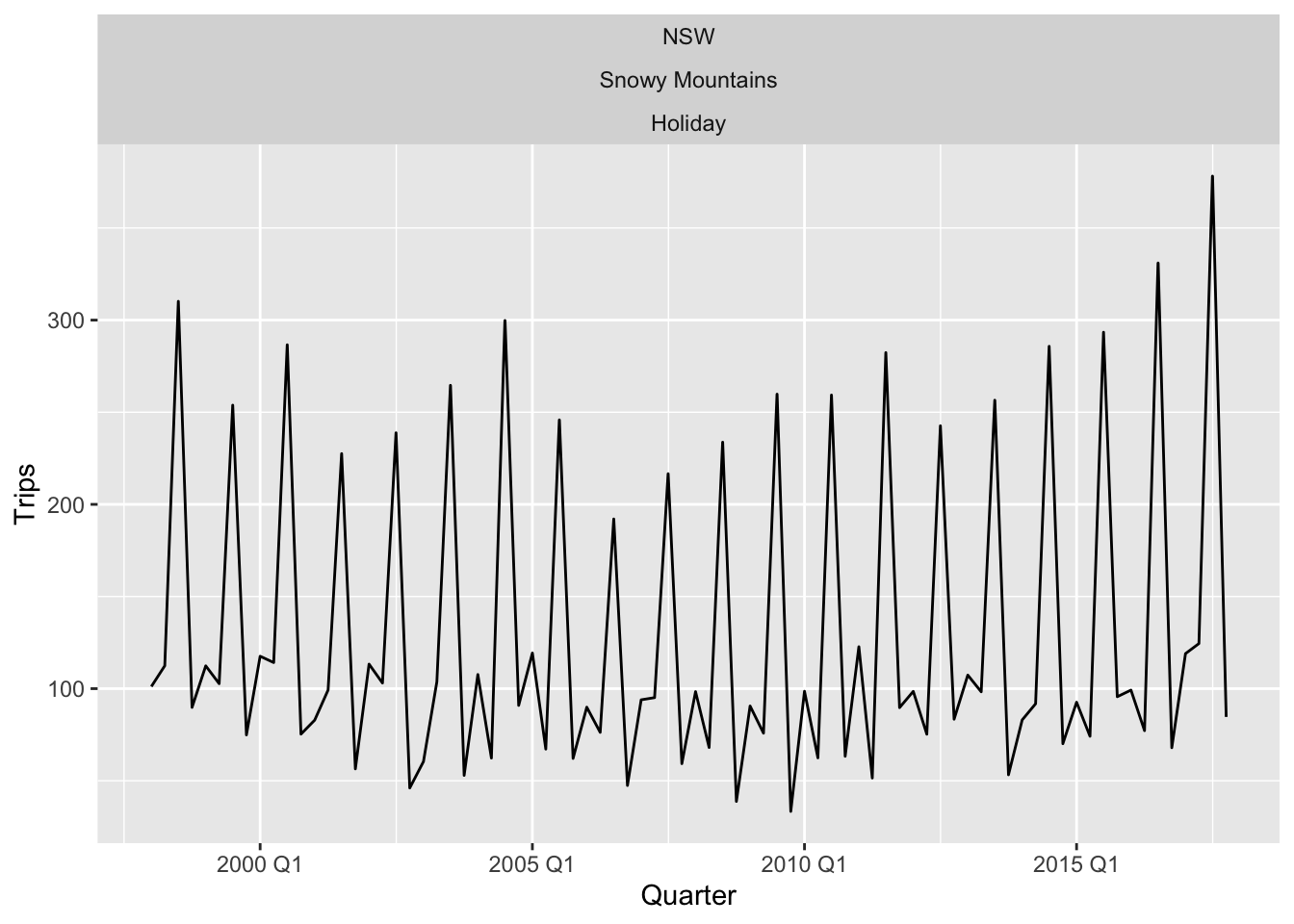
feat_stl() returns:
trend_strengthis strength of trendseasonal_strength_yearis strength of seasonalityseasonal_peak_yearindicates the timing of the peaksseasonal_trough_yearindicates the timing of the troughsspikinessmeasures the prevalence of spikes in the remainder componentlinearitymeasures the linearity of the trend componentcurvaturemeasures the curvature of the trend componentstl_e_acf1is the first autocorrelation coefficientstl_e_acf10is the sum of squares of the first ten autocorrelation coefficients
4.1.3 Other features
coef_hurstwill calculate the Hurst coefficient of a time series which is a measure of “long memory”. A series with long memory will have significant autocorrelations for many lags.
## # A tibble: 304 × 4
##    Region         State Purpose  coef_hurst
##    <chr>          <chr> <chr>         <dbl>
##  1 Adelaide       SA    Business      0.571
##  2 Adelaide       SA    Holiday       0.558
##  3 Adelaide       SA    Other         0.862
##  4 Adelaide       SA    Visiting      0.583
##  5 Adelaide Hills SA    Business      0.555
##  6 Adelaide Hills SA    Holiday       0.651
##  7 Adelaide Hills SA    Other         0.672
##  8 Adelaide Hills SA    Visiting      0.653
##  9 Alice Springs  NT    Business      0.713
## 10 Alice Springs  NT    Holiday       0.500
## # ℹ 294 more rows
Interpretation:
- \(H = 0.5\): The time series is a random walk with no memory (random behavior).
- \(H < 0.5\): The time series tends to reverse direction.
- \(H > 0.5\): The time series is persistent, meaning that if the series has been increasing, it is more likely to continue increasing, and if it has been decreasing, it is more likely to continue decreasing.
feat_spectralwill compute the (Shannon) spectral entropy of a time series, which is a measure of how easy the series is to forecast. A series which has strong trend and seasonality (and so is easy to forecast) will have entropy close to 0. A series that is very noisy (and so is difficult to forecast) will have entropy close to 1.
## # A tibble: 304 × 4
##    Region         State Purpose  spectral_entropy
##    <chr>          <chr> <chr>               <dbl>
##  1 Adelaide       SA    Business            0.843
##  2 Adelaide       SA    Holiday             0.753
##  3 Adelaide       SA    Other               0.793
##  4 Adelaide       SA    Visiting            0.768
##  5 Adelaide Hills SA    Business            0.991
##  6 Adelaide Hills SA    Holiday             0.928
##  7 Adelaide Hills SA    Other               0.913
##  8 Adelaide Hills SA    Visiting            1
##  9 Alice Springs  NT    Business            0.944
## 10 Alice Springs  NT    Holiday             0.544
## # ℹ 294 more rows
box_piercegives the Box-Pierce statistic for testing if a time series is white noise, and the corresponding p-value.
## # A tibble: 304 × 5
##    Region         State Purpose   bp_stat  bp_pvalue
##    <chr>          <chr> <chr>       <dbl>      <dbl>
##  1 Adelaide       SA    Business  0.0886  0.766
##  2 Adelaide       SA    Holiday   0.166   0.684
##  3 Adelaide       SA    Other    21.4     0.00000379
##  4 Adelaide       SA    Visiting  0.374   0.541
##  5 Adelaide Hills SA    Business  0.402   0.526
##  6 Adelaide Hills SA    Holiday   1.38    0.240
##  7 Adelaide Hills SA    Other     5.46    0.0195
##  8 Adelaide Hills SA    Visiting  1.55    0.213
##  9 Alice Springs  NT    Business  3.78    0.0518
## 10 Alice Springs  NT    Holiday   0.00349 0.953
## # ℹ 294 more rows
ljung_boxgives the Ljung-Box statistic for testing if a time series is white noise, and the corresponding p-value.
## # A tibble: 304 × 5
##    Region         State Purpose   lb_stat  lb_pvalue
##    <chr>          <chr> <chr>       <dbl>      <dbl>
##  1 Adelaide       SA    Business  0.0919  0.762
##  2 Adelaide       SA    Holiday   0.172   0.678
##  3 Adelaide       SA    Other    22.2     0.00000248
##  4 Adelaide       SA    Visiting  0.388   0.533
##  5 Adelaide Hills SA    Business  0.418   0.518
##  6 Adelaide Hills SA    Holiday   1.43    0.231
##  7 Adelaide Hills SA    Other     5.66    0.0173
##  8 Adelaide Hills SA    Visiting  1.61    0.205
##  9 Alice Springs  NT    Business  3.93    0.0476
## 10 Alice Springs  NT    Holiday   0.00362 0.952
## # ℹ 294 more rows
guerrerocomputes the optimal \(\lambda\) value for a Box-Cox transformation using the Guerrero method
## # A tibble: 304 × 4
##    Region         State Purpose  lambda_guerrero
##    <chr>          <chr> <chr>              <dbl>
##  1 Adelaide       SA    Business         0.514
##  2 Adelaide       SA    Holiday         -0.169
##  3 Adelaide       SA    Other           -0.227
##  4 Adelaide       SA    Visiting         0.870
##  5 Adelaide Hills SA    Business         0.124
##  6 Adelaide Hills SA    Holiday          0.246
##  7 Adelaide Hills SA    Other            0.365
##  8 Adelaide Hills SA    Visiting         0.00414
##  9 Alice Springs  NT    Business         0.561
## 10 Alice Springs  NT    Holiday          0.00174
## # ℹ 294 more rows
4.2 Exploring Australian tourism data
## # A tibble: 304 × 51
##    Region State Purpose trend_strength seasonal_strength_year seasonal_peak_year seasonal_trough_year spikiness linearity curvature stl_e_acf1 stl_e_acf10     acf1 acf10
##    <chr>  <chr> <chr>            <dbl>                  <dbl>              <dbl>                <dbl>     <dbl>     <dbl>     <dbl>      <dbl>       <dbl>    <dbl> <dbl>
##  1 Adela… SA    Busine…          0.464                  0.407                  3                    1   1.58e+2    -5.31     71.6       -0.532       0.594  0.0333  0.131
##  2 Adela… SA    Holiday          0.554                  0.619                  1                    2   9.17e+0    49.0      78.7       -0.510       0.561  0.0456  0.372
##  3 Adela… SA    Other            0.746                  0.202                  2                    1   2.10e+0    95.1      43.4       -0.351       0.403  0.517   1.15
##  4 Adela… SA    Visiti…          0.435                  0.452                  1                    3   5.61e+1    34.6      71.4       -0.501       1.01   0.0684  0.294
##  5 Adela… SA    Busine…          0.464                  0.179                  3                    0   1.03e-1     0.968    -3.22      -0.600       0.497  0.0709  0.134
##  6 Adela… SA    Holiday          0.528                  0.296                  2                    1   1.77e-1    10.5      24.0       -0.481       0.350  0.131   0.313
##  7 Adela… SA    Other            0.593                  0.404                  2                    2   4.44e-4     4.28      3.19      -0.298       0.281  0.261   0.330
##  8 Adela… SA    Visiti…          0.488                  0.254                  0                    3   6.50e+0    34.2      -0.529     -0.472       0.446  0.139   0.117
##  9 Alice… NT    Busine…          0.534                  0.251                  0                    1   1.69e-1    23.8      19.5       -0.492       0.548  0.217   0.367
## 10 Alice… NT    Holiday          0.381                  0.832                  3                    1   7.39e-1   -19.6      10.5       -0.522       0.726 -0.00660 2.11
## # ℹ 294 more rows
## # ℹ 37 more variables: diff1_acf1 <dbl>, diff1_acf10 <dbl>, diff2_acf1 <dbl>, diff2_acf10 <dbl>, season_acf1 <dbl>, pacf5 <dbl>, diff1_pacf5 <dbl>, diff2_pacf5 <dbl>,
## #   season_pacf <dbl>, zero_run_mean <dbl>, nonzero_squared_cv <dbl>, zero_start_prop <dbl>, zero_end_prop <dbl>, lambda_guerrero <dbl>, kpss_stat <dbl>,
## #   kpss_pvalue <dbl>, pp_stat <dbl>, pp_pvalue <dbl>, ndiffs <int>, nsdiffs <int>, bp_stat <dbl>, bp_pvalue <dbl>, lb_stat <dbl>, lb_pvalue <dbl>, var_tiled_var <dbl>,
## #   var_tiled_mean <dbl>, shift_level_max <dbl>, shift_level_index <dbl>, shift_var_max <dbl>, shift_var_index <dbl>, shift_kl_max <dbl>, shift_kl_index <dbl>,
## #   spectral_entropy <dbl>, n_crossing_points <int>, longest_flat_spot <int>, coef_hurst <dbl>, stat_arch_lm <dbl>
Provided the urca and fracdiff packages are installed, this gives 48 features for every combination of the three key variables (Region, State and Purpose). We can treat this tibble like any data set and analyse it to find interesting observations or groups of observations.
library(glue)
tourism_features |>
  select_at(vars(contains("season"), Purpose)) |>
  mutate(
    seasonal_peak_year = seasonal_peak_year +
      4*(seasonal_peak_year==0),
    seasonal_trough_year = seasonal_trough_year +
      4*(seasonal_trough_year==0),
    seasonal_peak_year = glue("Q{seasonal_peak_year}"),
    seasonal_trough_year = glue("Q{seasonal_trough_year}"),
  ) |>
  GGally::ggpairs(mapping = aes(colour = Purpose))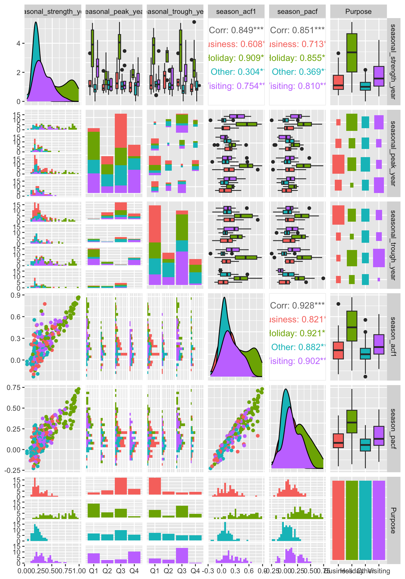
Using principal component method to reduce dimention and explore the variables.
library(broom)
pcs <- tourism_features |>
  select(-State, -Region, -Purpose) |>
  prcomp(scale = TRUE) |>
  augment(tourism_features)
pcs |>
  ggplot(aes(x = .fittedPC1, y = .fittedPC2, col = Purpose)) +
  geom_point() +
  theme(aspect.ratio = 1)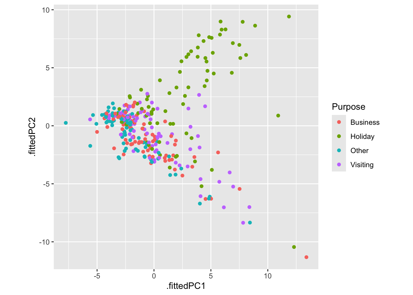
Explore outliers.
outliers <- pcs |>
  filter(.fittedPC1 > 10) |>
  select(Region, State, Purpose, .fittedPC1, .fittedPC2)
outliers
## # A tibble: 4 × 5
## Region State Purpose .fittedPC1 .fittedPC2
## <chr> <chr> <chr> <dbl> <dbl>
## 1 Australia's North West WA Business 13.4 -11.3
## 2 Australia's South West WA Holiday 10.9 0.880
## 3 Melbourne VIC Holiday 12.3 -10.4
## 4 South Coast NSW Holiday 11.9 9.42outliers |>
left_join(tourism, by = c("State", "Region", "Purpose"), multiple = "all") |>
mutate(Series = glue("{State}", "{Region}", "{Purpose}", .sep = "\n\n")) |>
ggplot(aes(x = Quarter, y = Trips)) +
geom_line() +
facet_grid(Series ~ ., scales = "free") +
labs(title = "Outlying time series in PC space")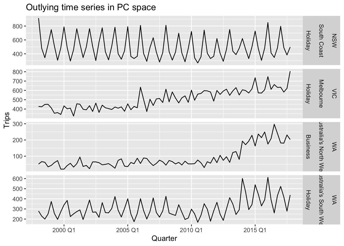
4.3 Exercises
?PBS

mean_sd <- function(x){
  c(mean=mean(x), sd = sd(x))
}

PBS |>
  features(Cost, mean_sd) |>
  filter(mean == max(mean)) |>
  left_join(PBS, by = c('Concession', 'Type', 'ATC1', 'ATC2'), multiple = "all") |>
  as_tsibble(index = Month, key = c('Concession', 'Type', 'ATC1', 'ATC2')) |>
  autoplot(Cost) +
  labs(title = 'Time series with the highest mean')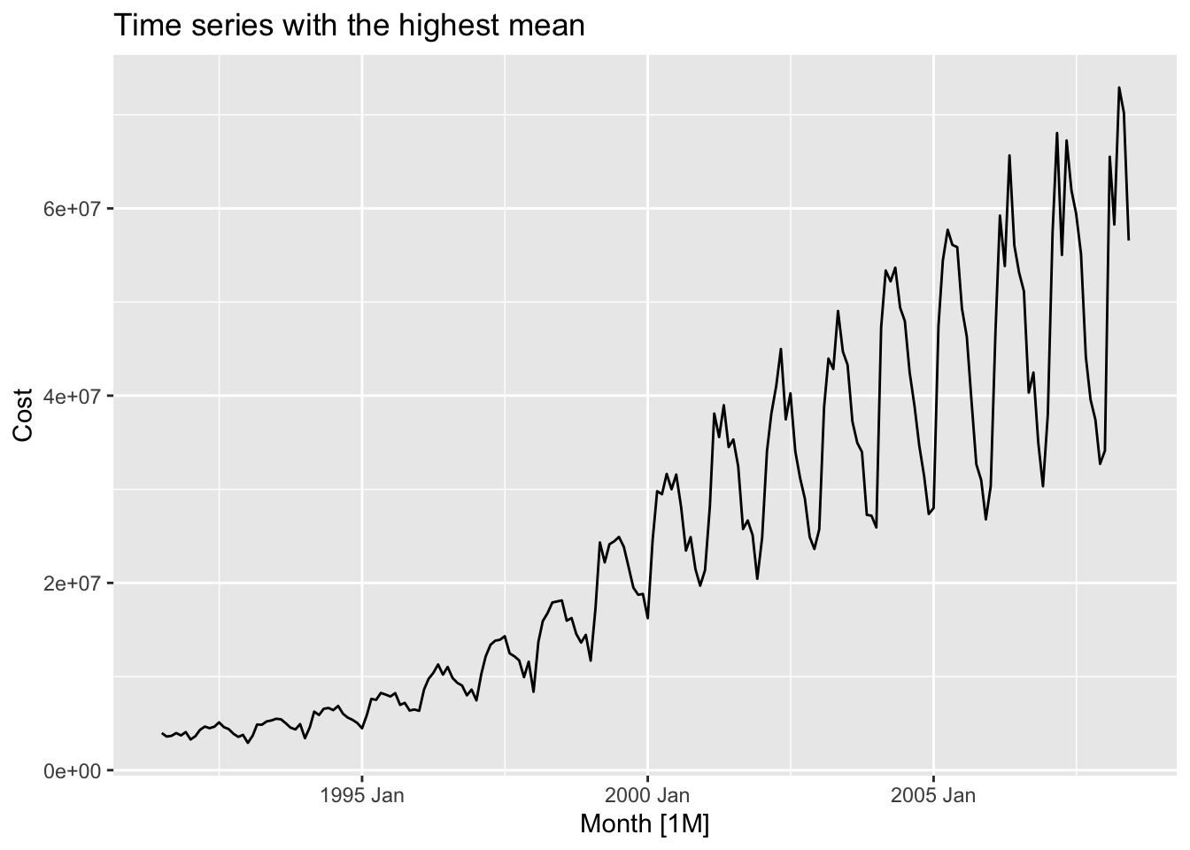
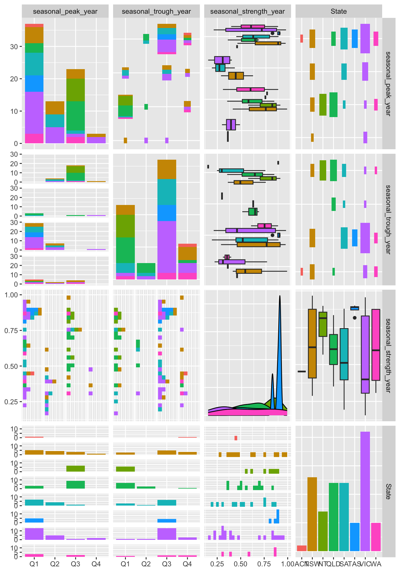
tourism |>
  filter(Purpose == 'Holiday') |>
  features(Trips, feature_set(pkgs = "feasts")) |>
  select_at(vars(contains("season"), State)) |>
  mutate(
    seasonal_peak_year = seasonal_peak_year +
      4*(seasonal_peak_year==0),
    seasonal_trough_year = seasonal_trough_year +
      4*(seasonal_trough_year==0),
    seasonal_peak_year = glue("Q{seasonal_peak_year}"),
    seasonal_trough_year = glue("Q{seasonal_trough_year}"),
  ) |>
  mutate(
    seasonal_peak_year = as.factor(seasonal_peak_year),
    seasonal_trough_year = as.factor(seasonal_trough_year)
  ) |>
  GGally::ggpairs(mapping = aes(colour = State),
                  columns = c("seasonal_peak_year",
                              "seasonal_trough_year",
                              "seasonal_strength_year",
                              "State"))