Chapter 2 Time series graphics

The source of the chapter

The first step in data analysis is to plot the data. Graphs help visualize patterns, outliers, trends, and relationships. These insights guide the choice of forecasting methods and appropriate graphs, depending on the data type.

# loading libraries
library(tsibble)
library(tsibbledata)
library(tidyverse)
# to read data
library(rio)
library(ggplot2)
library(fabletools)
library(feasts)
library(fpp3)

2.1 tsibble object

The source of the section

2.1.1 The index variable

y <- tsibble(Year = 2015:2019,
             Observations = c(123, 39, 78, 52, 110),
             index = Year)

y

## # A tsibble: 5 x 2 [1Y]
##    Year Observations
##   <int>        <dbl>
## 1  2015          123
## 2  2016           39
## 3  2017           78
## 4  2018           52
## 5  2019          110

# the structure of the tsibble
str(y)

## tbl_ts [5 × 2] (S3: tbl_ts/tbl_df/tbl/data.frame)
##  $ Year        : int [1:5] 2015 2016 2017 2018 2019
##  $ Observations: num [1:5] 123 39 78 52 110
##  - attr(*, "key")= tibble [1 × 1] (S3: tbl_df/tbl/data.frame)
##   ..$ .rows: list<int> [1:1] 
##   .. ..$ : int [1:5] 1 2 3 4 5
##   .. ..@ ptype: int(0) 
##  - attr(*, "index")= chr "Year"
##   ..- attr(*, "ordered")= logi TRUE
##  - attr(*, "index2")= chr "Year"
##  - attr(*, "interval")= interval [1:1] 1Y
##   ..@ .regular: logi TRUE

Convert from data frame (or tibble) to tsibble.

df <- data.frame(Month = as.character(make_yearmonth(year = 2024, month = 1:5)),
                 Observation = c(123, 45, 32, 54, 22))
df                 

##      Month Observation
## 1 2024 Jan         123
## 2 2024 Feb          45
## 3 2024 Mar          32
## 4 2024 Apr          54
## 5 2024 May          22

df |>
  mutate(Month = yearmonth(Month)) |>
  as_tsibble(index = Month)

## # A tsibble: 5 x 2 [1M]
##      Month Observation
##      <mth>       <dbl>
## 1 2024 Jan         123
## 2 2024 Feb          45
## 3 2024 Mar          32
## 4 2024 Apr          54
## 5 2024 May          22

[1M] indicates a monthly data.

To convert tsibble to old ts format:

df2 <- df |> as.ts()

df2

## Time Series:
## Start = 1 
## End = 5 
## Frequency = 1 
##   Month Observation
## 1     3         123
## 2     2          45
## 3     4          32
## 4     1          54
## 5     5          22

To convert from ts to tsibble:

AirPassengers

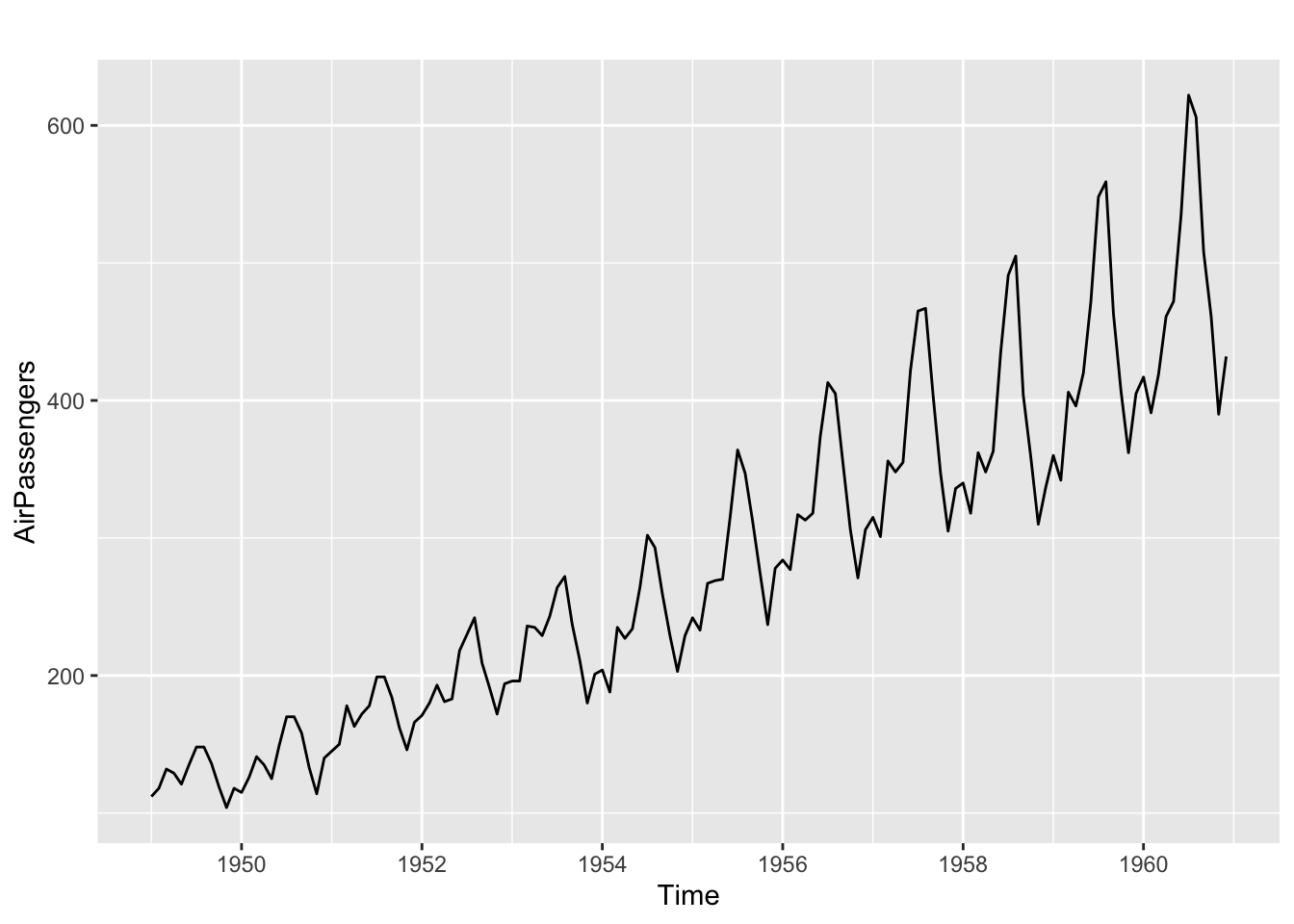
##      Jan Feb Mar Apr May Jun Jul Aug Sep Oct Nov Dec
## 1949 112 118 132 129 121 135 148 148 136 119 104 118
## 1950 115 126 141 135 125 149 170 170 158 133 114 140
## 1951 145 150 178 163 172 178 199 199 184 162 146 166
## 1952 171 180 193 181 183 218 230 242 209 191 172 194
## 1953 196 196 236 235 229 243 264 272 237 211 180 201
## 1954 204 188 235 227 234 264 302 293 259 229 203 229
## 1955 242 233 267 269 270 315 364 347 312 274 237 278
## 1956 284 277 317 313 318 374 413 405 355 306 271 306
## 1957 315 301 356 348 355 422 465 467 404 347 305 336
## 1958 340 318 362 348 363 435 491 505 404 359 310 337
## 1959 360 342 406 396 420 472 548 559 463 407 362 405
## 1960 417 391 419 461 472 535 622 606 508 461 390 432

AirPassengers |>
  as_tsibble() |> # creates index column fot time point
  rename(month = index)

## # A tsibble: 144 x 2 [1M]
##       month value
##       <mth> <dbl>
##  1 1949 Jan   112
##  2 1949 Feb   118
##  3 1949 Mar   132
##  4 1949 Apr   129
##  5 1949 May   121
##  6 1949 Jun   135
##  7 1949 Jul   148
##  8 1949 Aug   148
##  9 1949 Sep   136
## 10 1949 Oct   119
## # ℹ 134 more rows

2.1.2 The key variable

Multiple time series in a single object.

olympic_running

## # A tsibble: 312 x 4 [4Y]
## # Key:       Length, Sex [14]
##     Year Length Sex    Time
##    <int>  <int> <chr> <dbl>
##  1  1896    100 men    12  
##  2  1900    100 men    11  
##  3  1904    100 men    11  
##  4  1908    100 men    10.8
##  5  1912    100 men    10.8
##  6  1916    100 men    NA  
##  7  1920    100 men    10.8
##  8  1924    100 men    10.6
##  9  1928    100 men    10.8
## 10  1932    100 men    10.3
## # ℹ 302 more rows

[4K] indicates that the interval if these observations is every four years. [14] indicates there are 14 separaste time series in the stibble object.

key(olympic_running)

## [[1]]
## Length
## 
## [[2]]
## Sex

print(olympic_running |> distinct(Sex))

## # A tibble: 2 × 1
##   Sex  
##   <chr>
## 1 men  
## 2 women

print(olympic_running |> distinct(Length))

## # A tibble: 7 × 1
##   Length
##    <int>
## 1    100
## 2    200
## 3    400
## 4    800
## 5   1500
## 6   5000
## 7  10000

print(olympic_running |> distinct(Sex, Length))

## # A tibble: 14 × 2
##    Sex   Length
##    <chr>  <int>
##  1 men      100
##  2 women    100
##  3 men      200
##  4 women    200
##  5 men      400
##  6 women    400
##  7 men      800
##  8 women    800
##  9 men     1500
## 10 women   1500
## 11 men     5000
## 12 women   5000
## 13 men    10000
## 14 women  10000

key_vars(olympic_running)

## [1] "Length" "Sex"

2.1.3 Working with tsibble object

dplyr functions such as mutate(), filter(), select() and summarise() work with tsibble objects.

PBS

## # A tsibble: 67,596 x 9 [1M]
## # Key:       Concession, Type, ATC1, ATC2 [336]
##       Month Concession   Type        ATC1  ATC1_desc                       ATC2  ATC2_desc                   Scripts  Cost
##       <mth> <chr>        <chr>       <chr> <chr>                           <chr> <chr>                         <dbl> <dbl>
##  1 1991 Jul Concessional Co-payments A     Alimentary tract and metabolism A01   STOMATOLOGICAL PREPARATIONS   18228 67877
##  2 1991 Aug Concessional Co-payments A     Alimentary tract and metabolism A01   STOMATOLOGICAL PREPARATIONS   15327 57011
##  3 1991 Sep Concessional Co-payments A     Alimentary tract and metabolism A01   STOMATOLOGICAL PREPARATIONS   14775 55020
##  4 1991 Oct Concessional Co-payments A     Alimentary tract and metabolism A01   STOMATOLOGICAL PREPARATIONS   15380 57222
##  5 1991 Nov Concessional Co-payments A     Alimentary tract and metabolism A01   STOMATOLOGICAL PREPARATIONS   14371 52120
##  6 1991 Dec Concessional Co-payments A     Alimentary tract and metabolism A01   STOMATOLOGICAL PREPARATIONS   15028 54299
##  7 1992 Jan Concessional Co-payments A     Alimentary tract and metabolism A01   STOMATOLOGICAL PREPARATIONS   11040 39753
##  8 1992 Feb Concessional Co-payments A     Alimentary tract and metabolism A01   STOMATOLOGICAL PREPARATIONS   15165 54405
##  9 1992 Mar Concessional Co-payments A     Alimentary tract and metabolism A01   STOMATOLOGICAL PREPARATIONS   16898 61108
## 10 1992 Apr Concessional Co-payments A     Alimentary tract and metabolism A01   STOMATOLOGICAL PREPARATIONS   18141 65356
## # ℹ 67,586 more rows

PBS |>
  filter(ATC2 == 'A10')

## # A tsibble: 816 x 9 [1M]
## # Key:       Concession, Type, ATC1, ATC2 [4]
##       Month Concession   Type        ATC1  ATC1_desc                       ATC2  ATC2_desc            Scripts    Cost
##       <mth> <chr>        <chr>       <chr> <chr>                           <chr> <chr>                  <dbl>   <dbl>
##  1 1991 Jul Concessional Co-payments A     Alimentary tract and metabolism A10   ANTIDIABETIC THERAPY   89733 2092878
##  2 1991 Aug Concessional Co-payments A     Alimentary tract and metabolism A10   ANTIDIABETIC THERAPY   77101 1795733
##  3 1991 Sep Concessional Co-payments A     Alimentary tract and metabolism A10   ANTIDIABETIC THERAPY   76255 1777231
##  4 1991 Oct Concessional Co-payments A     Alimentary tract and metabolism A10   ANTIDIABETIC THERAPY   78681 1848507
##  5 1991 Nov Concessional Co-payments A     Alimentary tract and metabolism A10   ANTIDIABETIC THERAPY   70554 1686458
##  6 1991 Dec Concessional Co-payments A     Alimentary tract and metabolism A10   ANTIDIABETIC THERAPY   75814 1843079
##  7 1992 Jan Concessional Co-payments A     Alimentary tract and metabolism A10   ANTIDIABETIC THERAPY   64186 1564702
##  8 1992 Feb Concessional Co-payments A     Alimentary tract and metabolism A10   ANTIDIABETIC THERAPY   75899 1732508
##  9 1992 Mar Concessional Co-payments A     Alimentary tract and metabolism A10   ANTIDIABETIC THERAPY   89445 2046102
## 10 1992 Apr Concessional Co-payments A     Alimentary tract and metabolism A10   ANTIDIABETIC THERAPY   97315 2225977
## # ℹ 806 more rows

PBS |>
  filter(ATC2 == 'A10') |>
  select(Month, Concession, Type, Cost)

## # A tsibble: 816 x 4 [1M]
## # Key:       Concession, Type [4]
##       Month Concession   Type           Cost
##       <mth> <chr>        <chr>         <dbl>
##  1 1991 Jul Concessional Co-payments 2092878
##  2 1991 Aug Concessional Co-payments 1795733
##  3 1991 Sep Concessional Co-payments 1777231
##  4 1991 Oct Concessional Co-payments 1848507
##  5 1991 Nov Concessional Co-payments 1686458
##  6 1991 Dec Concessional Co-payments 1843079
##  7 1992 Jan Concessional Co-payments 1564702
##  8 1992 Feb Concessional Co-payments 1732508
##  9 1992 Mar Concessional Co-payments 2046102
## 10 1992 Apr Concessional Co-payments 2225977
## # ℹ 806 more rows

print(index_var(PBS))

## [1] "Month"

print(key_vars(PBS))

## [1] "Concession" "Type"       "ATC1"       "ATC2"

If no one index or key were not explicitly selected, they would be returned as they are required for tsibble to ensure each row contains a unique combination of keys and index.

PBS |>
  filter(ATC2 == 'A10') |>
  select(Cost)

## # A tsibble: 816 x 6 [1M]
## # Key:       Concession, Type, ATC1, ATC2 [4]
##       Cost    Month Concession   Type        ATC1  ATC2 
##      <dbl>    <mth> <chr>        <chr>       <chr> <chr>
##  1 2092878 1991 Jul Concessional Co-payments A     A10  
##  2 1795733 1991 Aug Concessional Co-payments A     A10  
##  3 1777231 1991 Sep Concessional Co-payments A     A10  
##  4 1848507 1991 Oct Concessional Co-payments A     A10  
##  5 1686458 1991 Nov Concessional Co-payments A     A10  
##  6 1843079 1991 Dec Concessional Co-payments A     A10  
##  7 1564702 1992 Jan Concessional Co-payments A     A10  
##  8 1732508 1992 Feb Concessional Co-payments A     A10  
##  9 2046102 1992 Mar Concessional Co-payments A     A10  
## 10 2225977 1992 Apr Concessional Co-payments A     A10  
## # ℹ 806 more rows

PBS |>
  filter(ATC2 == 'A10') |>
  select(Concession, Type, Cost)

## # A tsibble: 816 x 4 [1M]
## # Key:       Concession, Type [4]
##    Concession   Type           Cost    Month
##    <chr>        <chr>         <dbl>    <mth>
##  1 Concessional Co-payments 2092878 1991 Jul
##  2 Concessional Co-payments 1795733 1991 Aug
##  3 Concessional Co-payments 1777231 1991 Sep
##  4 Concessional Co-payments 1848507 1991 Oct
##  5 Concessional Co-payments 1686458 1991 Nov
##  6 Concessional Co-payments 1843079 1991 Dec
##  7 Concessional Co-payments 1564702 1992 Jan
##  8 Concessional Co-payments 1732508 1992 Feb
##  9 Concessional Co-payments 2046102 1992 Mar
## 10 Concessional Co-payments 2225977 1992 Apr
## # ℹ 806 more rows

PBS |>
  filter(ATC2 == 'A10') |>
  select(Month, Concession, Type, Cost) |>
  summarise(TotalC = sum(Cost))

## # A tsibble: 204 x 2 [1M]
##       Month  TotalC
##       <mth>   <dbl>
##  1 1991 Jul 3526591
##  2 1991 Aug 3180891
##  3 1991 Sep 3252221
##  4 1991 Oct 3611003
##  5 1991 Nov 3565869
##  6 1991 Dec 4306371
##  7 1992 Jan 5088335
##  8 1992 Feb 2814520
##  9 1992 Mar 2985811
## 10 1992 Apr 3204780
## # ℹ 194 more rows

PBS |>
  filter(ATC2 == 'A10') |>
  select(Month, Concession, Type, Cost) |>
  summarise(TotalC = sum(Cost)) |>
  mutate(Cost = TotalC / 1e6)

## # A tsibble: 204 x 3 [1M]
##       Month  TotalC  Cost
##       <mth>   <dbl> <dbl>
##  1 1991 Jul 3526591  3.53
##  2 1991 Aug 3180891  3.18
##  3 1991 Sep 3252221  3.25
##  4 1991 Oct 3611003  3.61
##  5 1991 Nov 3565869  3.57
##  6 1991 Dec 4306371  4.31
##  7 1992 Jan 5088335  5.09
##  8 1992 Feb 2814520  2.81
##  9 1992 Mar 2985811  2.99
## 10 1992 Apr 3204780  3.20
## # ℹ 194 more rows

Save to the further usage.

PBS |>
  filter(ATC2 == 'A10') |>
  select(Month, Concession, Type, Cost) |>
  summarise(TotalC = sum(Cost)) |>
  mutate(Cost = TotalC / 1e6) -> a10

a10

## # A tsibble: 204 x 3 [1M]
##       Month  TotalC  Cost
##       <mth>   <dbl> <dbl>
##  1 1991 Jul 3526591  3.53
##  2 1991 Aug 3180891  3.18
##  3 1991 Sep 3252221  3.25
##  4 1991 Oct 3611003  3.61
##  5 1991 Nov 3565869  3.57
##  6 1991 Dec 4306371  4.31
##  7 1992 Jan 5088335  5.09
##  8 1992 Feb 2814520  2.81
##  9 1992 Mar 2985811  2.99
## 10 1992 Apr 3204780  3.20
## # ℹ 194 more rows

2.1.4 Read a csv file and convert to a tsibble

prison <- import('https://OTexts.com/fpp3/extrafiles/prison_population.csv')

prison <- prison |>
  mutate(Quarter = yearquarter(Date)) |>
  select(-Date) |>
  as_tsibble(key = c(State, Gender, Legal, Indigenous))

## Using `Quarter` as index variable.

prison

## # A tsibble: 3,072 x 6 [1Q]
## # Key:       State, Gender, Legal, Indigenous [64]
##    State Gender Legal    Indigenous Count Quarter
##    <chr> <chr>  <chr>    <chr>      <int>   <qtr>
##  1 ACT   Female Remanded ATSI           0 2005 Q1
##  2 ACT   Female Remanded ATSI           1 2005 Q2
##  3 ACT   Female Remanded ATSI           0 2005 Q3
##  4 ACT   Female Remanded ATSI           0 2005 Q4
##  5 ACT   Female Remanded ATSI           1 2006 Q1
##  6 ACT   Female Remanded ATSI           1 2006 Q2
##  7 ACT   Female Remanded ATSI           1 2006 Q3
##  8 ACT   Female Remanded ATSI           0 2006 Q4
##  9 ACT   Female Remanded ATSI           0 2007 Q1
## 10 ACT   Female Remanded ATSI           1 2007 Q2
## # ℹ 3,062 more rows

For a tsibble to be valid, it requires a unique index for each combination of keys. The tsibble() or as_tsibble() function will return an error if this is not true.

2.1.5 The seasonal period

The seasonal period is the number of observations before the seasonal pattern repeats.

Data	Minute	Hour	Day	Week	Year
Quarters					4
Months					12
Weeks					52.18
Days				7	365.25
Hours			24	168	8766
Minutes		60	1440	10080	525960
Seconds	60	3600	86400	604800	31557600

2.2 Time plot

The source of the section

a10

## # A tsibble: 204 x 3 [1M]
##       Month  TotalC  Cost
##       <mth>   <dbl> <dbl>
##  1 1991 Jul 3526591  3.53
##  2 1991 Aug 3180891  3.18
##  3 1991 Sep 3252221  3.25
##  4 1991 Oct 3611003  3.61
##  5 1991 Nov 3565869  3.57
##  6 1991 Dec 4306371  4.31
##  7 1992 Jan 5088335  5.09
##  8 1992 Feb 2814520  2.81
##  9 1992 Mar 2985811  2.99
## 10 1992 Apr 3204780  3.20
## # ℹ 194 more rows

autoplot() is a smart function.

It automatically produces an appropriate plot of whatever you pass to it in the first argument

a10 |> 
  autoplot(Cost) +
  labs(y='$ (millions)', title = 'Australian antidiabetic drug sales')

Using ggplot.

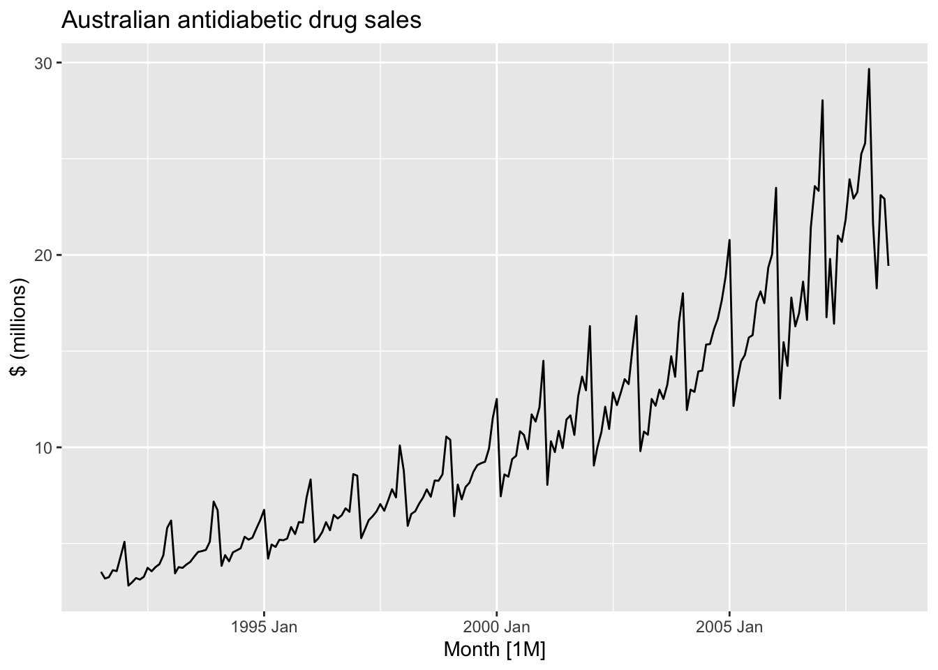
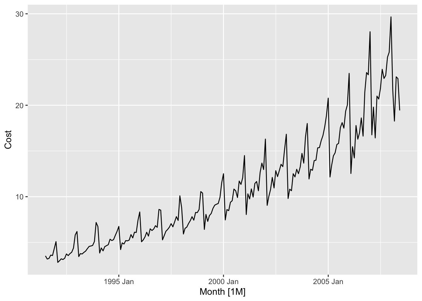
a10 |>
  ggplot(aes(x = Month, y = Cost)) +
    geom_line() +
    ggtitle('Australian antidiabetic drug sales') +
    ylab('$ (millions)')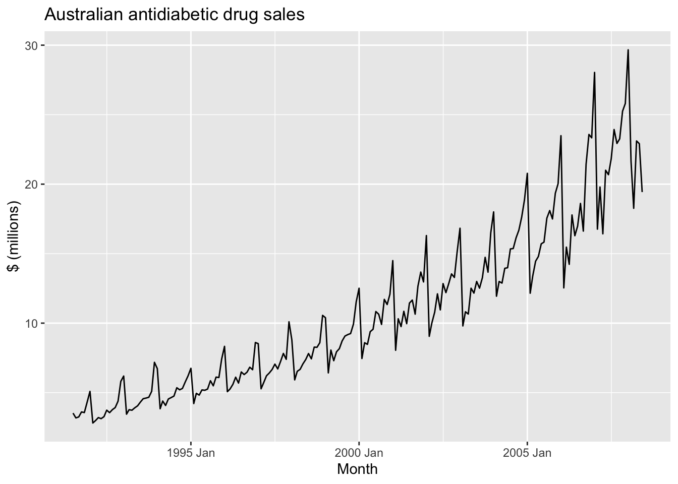

Add points on the line.

a10 |> 
  autoplot(Cost) +
  geom_point() +
  labs(y='$ (millions)', title = 'Australian antidiabetic drug sales')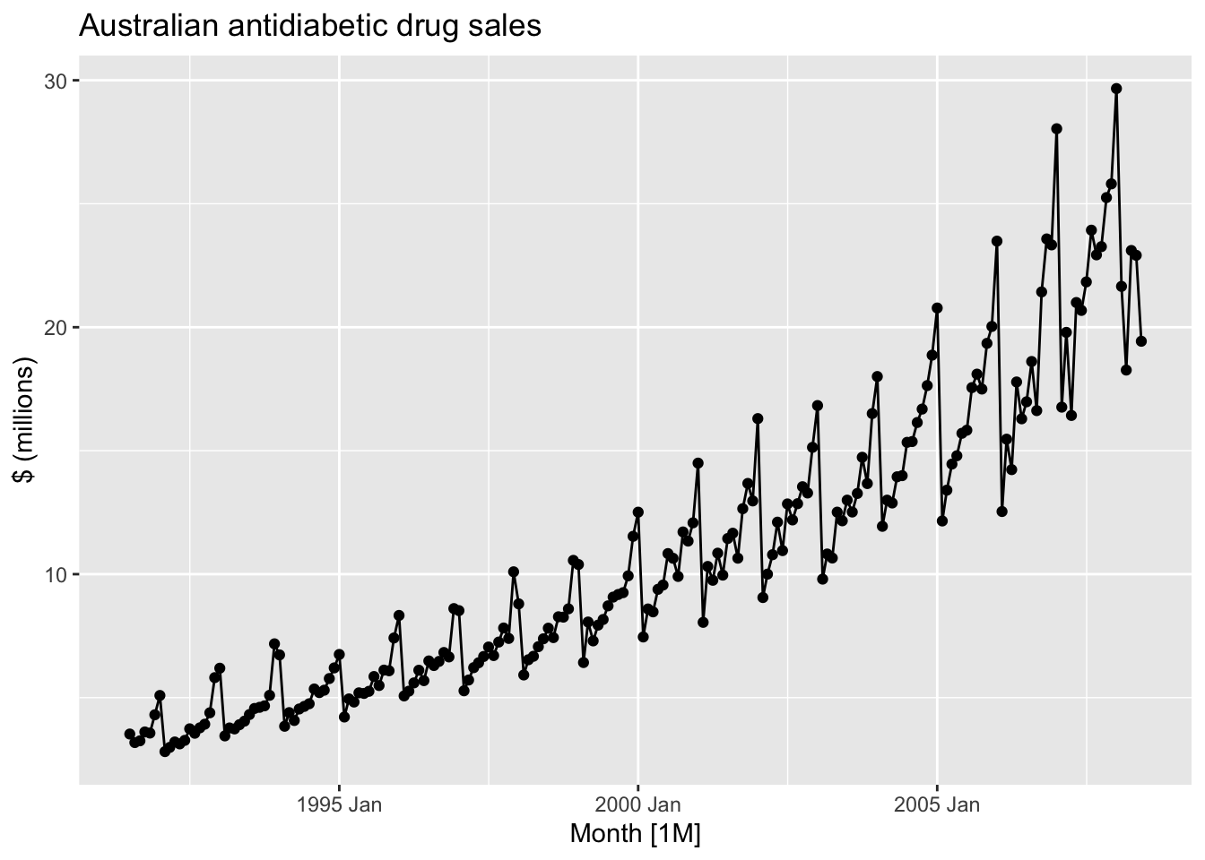

ansett

## # A tsibble: 7,407 x 4 [1W]
## # Key:       Airports, Class [30]
##        Week Airports Class    Passengers
##      <week> <chr>    <chr>         <dbl>
##  1 1989 W28 ADL-PER  Business        193
##  2 1989 W29 ADL-PER  Business        254
##  3 1989 W30 ADL-PER  Business        185
##  4 1989 W31 ADL-PER  Business        254
##  5 1989 W32 ADL-PER  Business        191
##  6 1989 W33 ADL-PER  Business        136
##  7 1989 W34 ADL-PER  Business          0
##  8 1989 W35 ADL-PER  Business          0
##  9 1989 W36 ADL-PER  Business          0
## 10 1989 W37 ADL-PER  Business          0
## # ℹ 7,397 more rows

ansett |>
  autoplot(Passengers)

Distinct categories.

print(ansett |> distinct(Class))

## # A tibble: 3 × 1
##   Class   
##   <chr>   
## 1 Business
## 2 Economy 
## 3 First

print(ansett |> distinct(Airports))

## # A tibble: 10 × 1
##    Airports
##    <chr>   
##  1 ADL-PER 
##  2 MEL-ADL 
##  3 MEL-BNE 
##  4 MEL-OOL 
##  5 MEL-PER 
##  6 MEL-SYD 
##  7 SYD-ADL 
##  8 SYD-BNE 
##  9 SYD-OOL 
## 10 SYD-PER

ansett |>
  filter(Class == 'Economy') |>
  autoplot(Passengers) +
  labs(y = 'Number of passanger', x = 'Week', title = 'Number of passangers by routs')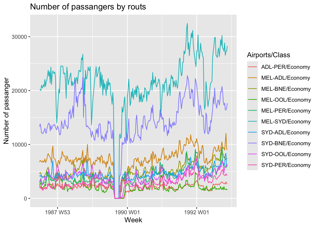

ansett |>
  filter(Airports == 'MEL-SYD') |>
  select(-Airports) |> # to avoid the filtered rout from titles
  autoplot(Passengers) +
  labs(y = 'Number of passanger', x = 'Week', title = 'Number of passangers by class')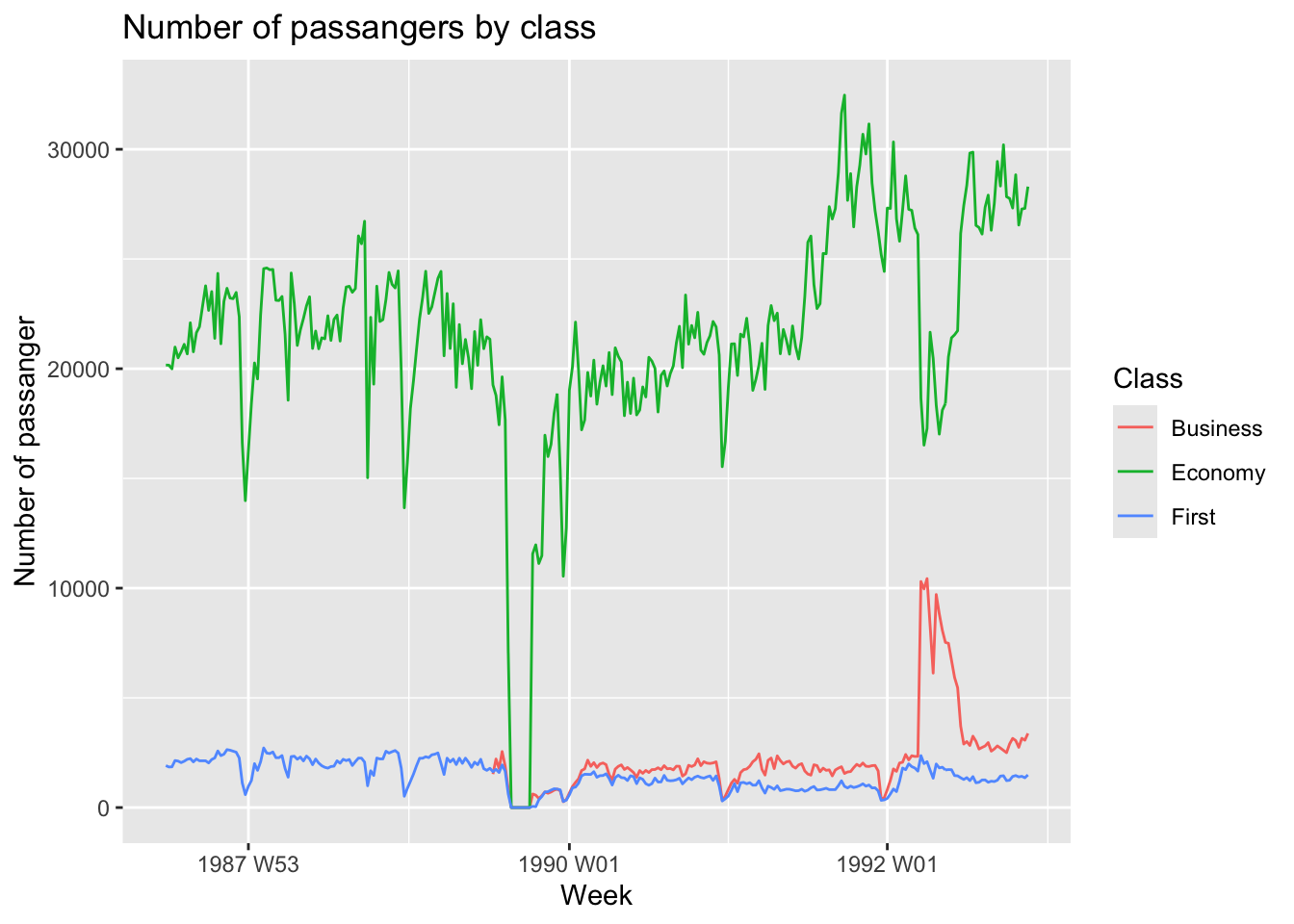

melsyd_economy <- ansett |>
  filter(Airports == 'MEL-SYD', Class == 'Economy') |>
  mutate(Passengers = Passengers/1e3)

melsyd_economy |>
  autoplot(Passengers) +
  labs(title = 'Ansett airlines economy class',
       subtitle = 'Melbourne-Sydney',
       y = 'Passangers (K)', x = 'Week')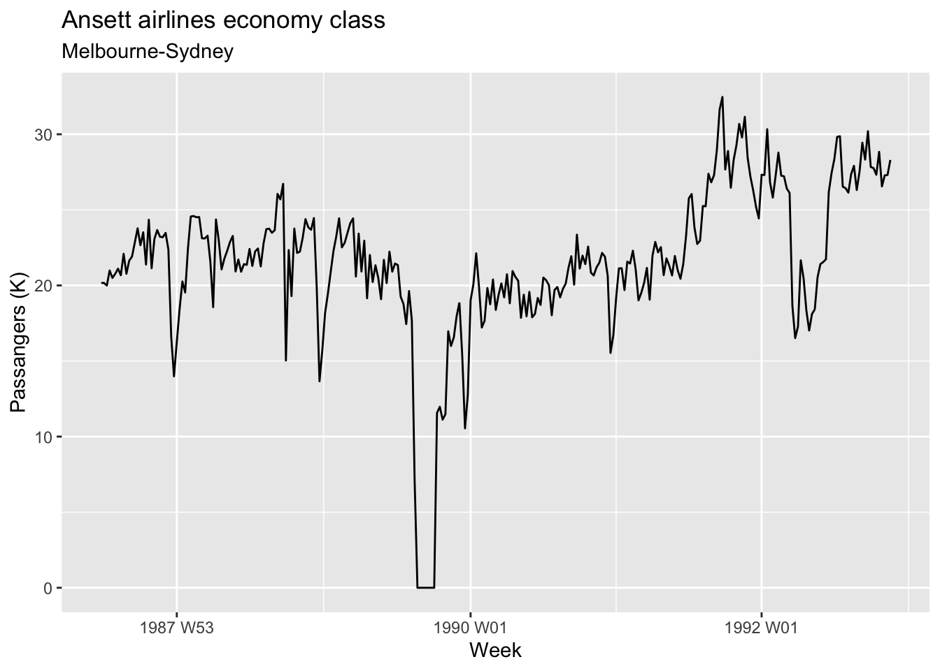

2.3 Time series patterns

The source of the section

• Trend: pattern exists when there is a long-term increase or decrease in the data.
• Seasonal: pattern exists when a series is influenced by seasonal factor (quarter, month, week, day of the week, etc.).
• Cyclic: pattern exists when data exhibit rises and falls that are not of fixed period.

# positive trend
aus_production |>
  filter(year(Quarter) >= 1980) |>
  autoplot(Electricity) +
  labs(y = 'GWh', title = 'Australian electricity production')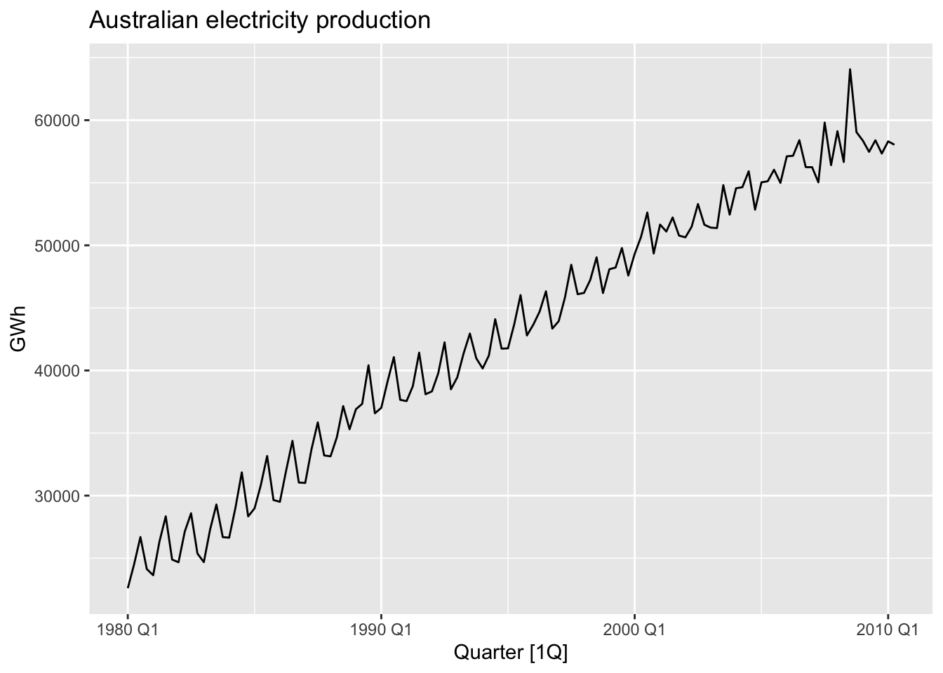

Important! Many time series include trend, cycles and seasonality. When choosing a forecasting method, we will first need to identify the time series patterns in the data, and then choose a method that is able to capture the patterns properly.

aus_production |>
  autoplot(Bricks) +
  labs(y = 'MIllion units', title = 'Australian clay brick production')

## Warning: Removed 20 rows containing missing values or values outside the scale range (`geom_line()`).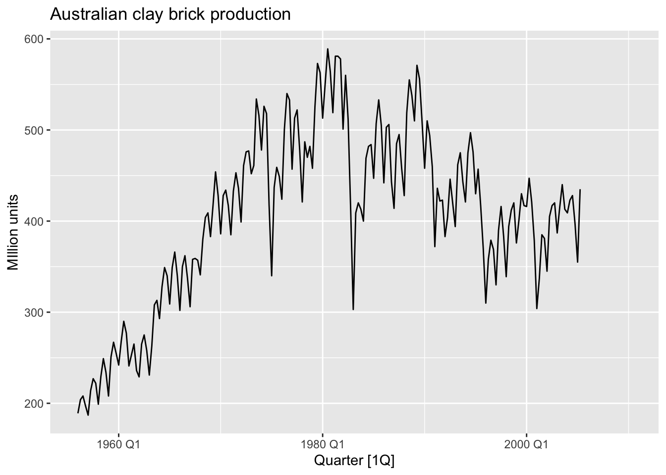

The timing of peaks and troughs is predictable with seasonal data, but unpredictable in the long term with ciclic data.

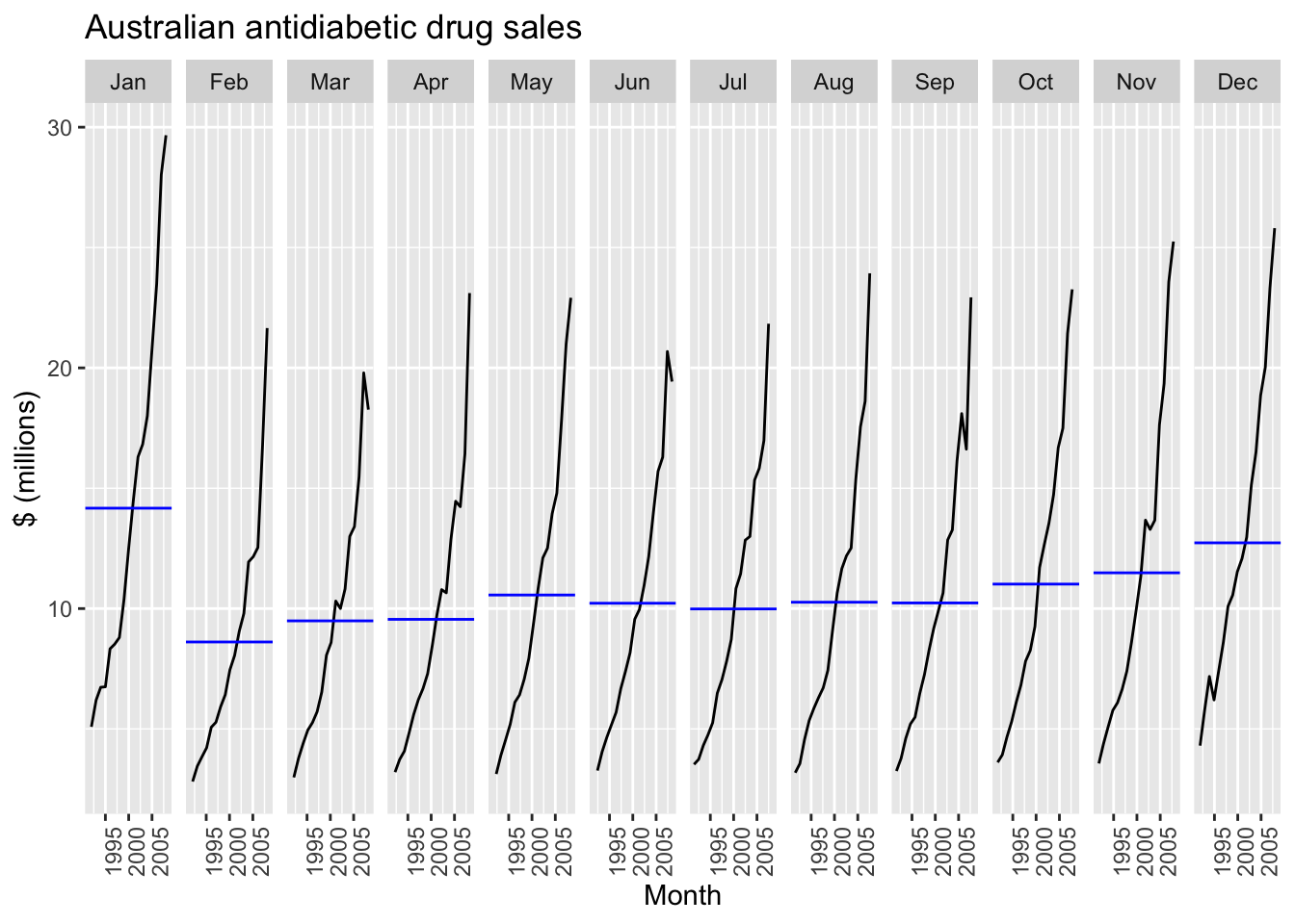
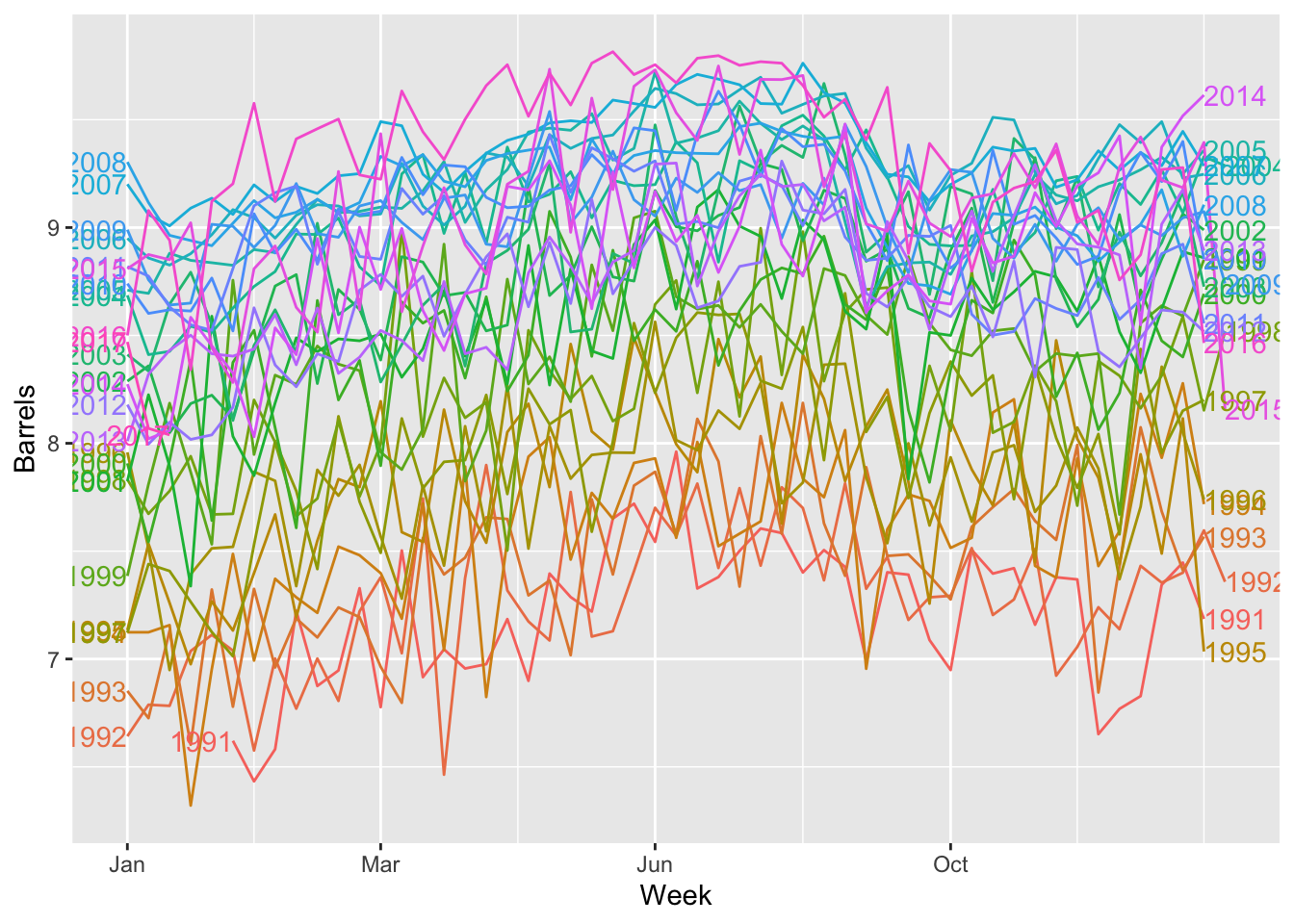
2.4 Seasonal plots

The source of the section

a10 |> 
  autoplot(Cost)

A seasonal plot plots the data against the individual season in which the data were observed.

a10 |>
  gg_season(Cost, labels = 'both') +
  labs(y = '$ million', title = 'Seasonal plot: antidiabetic drug sales')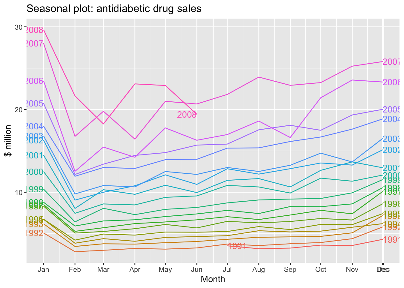

beer <- aus_production |>
  select(Quarter, Beer) |>
  filter(year(Quarter) >= 1992)

beer |> autoplot(Beer) +
  geom_point() +
  labs(title = 'Australian beer production', y = 'Megalitres')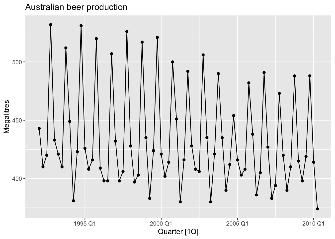

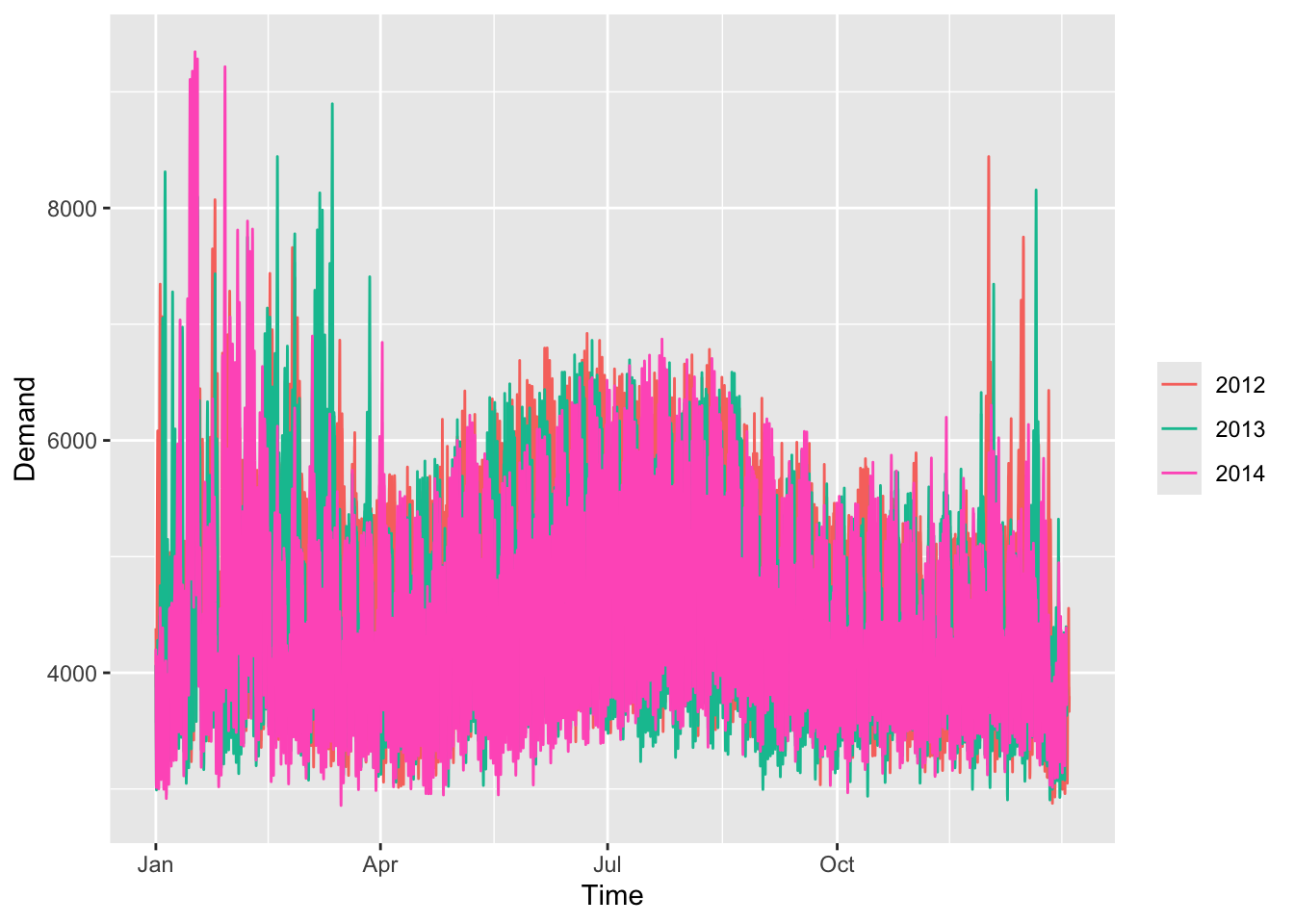
2.4.1 Multiple seasonal periods

vic_elec |> autoplot()

## Plot variable not specified, automatically selected `.vars = Demand`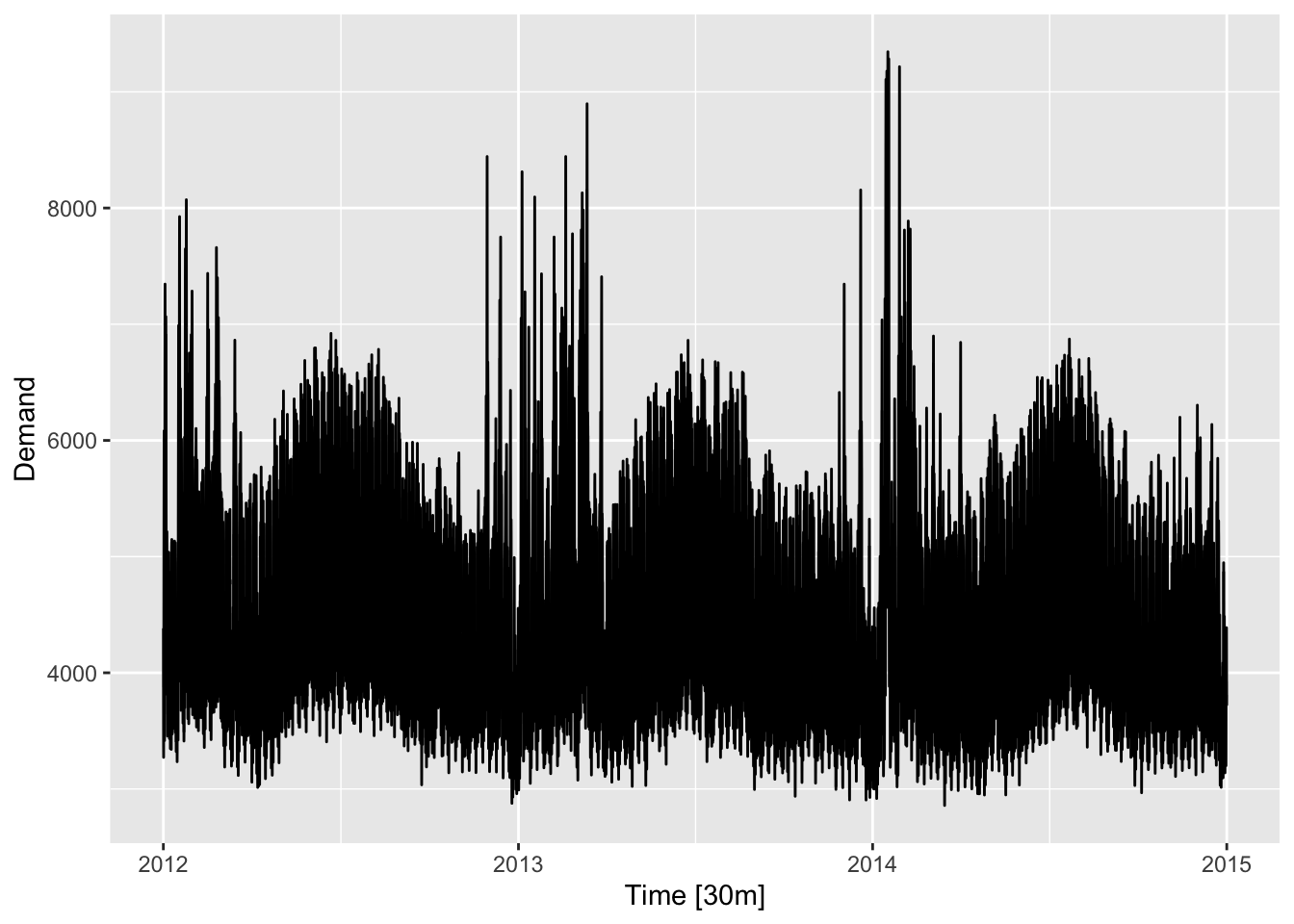

vic_elec |>
  gg_season(Demand)

By time during the day.

vic_elec |>
  gg_season(Demand, period = 'day') +
  theme(legend.position = "none") +
  labs(y="MWh", title="Electricity demand: Victoria")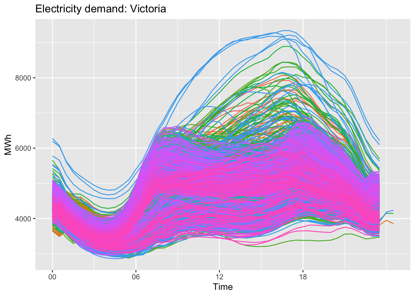

Weekly.

vic_elec |>
  gg_season(Demand, period = 'week') +
  theme(legend.position = "none") +
  labs(y="MWh", title="Electricity demand: Victoria")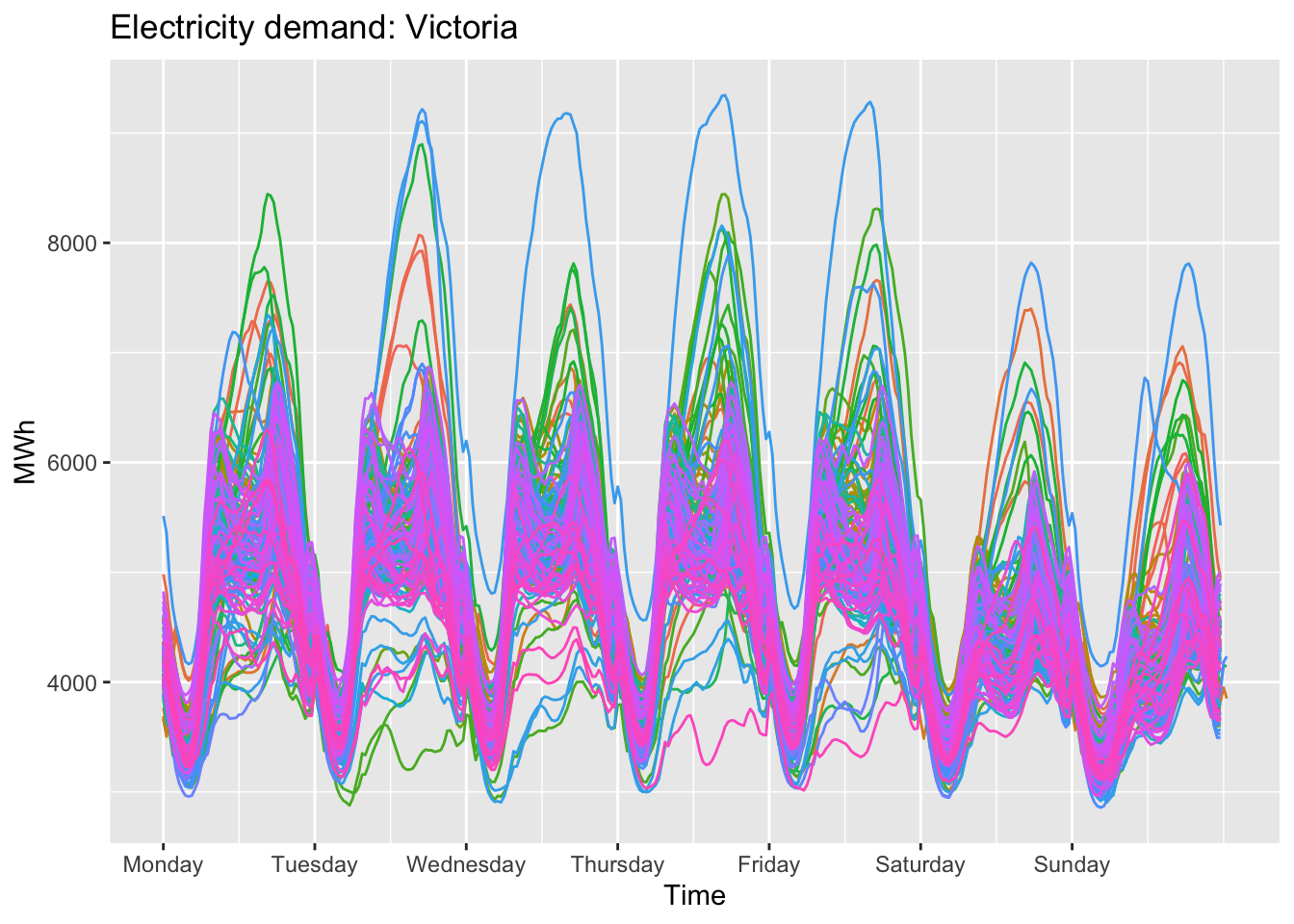

Monthly.

vic_elec |>
  gg_season(Demand, period = 'month') +
  theme(legend.position = "none") +
  labs(y="MWh", title="Electricity demand: Victoria")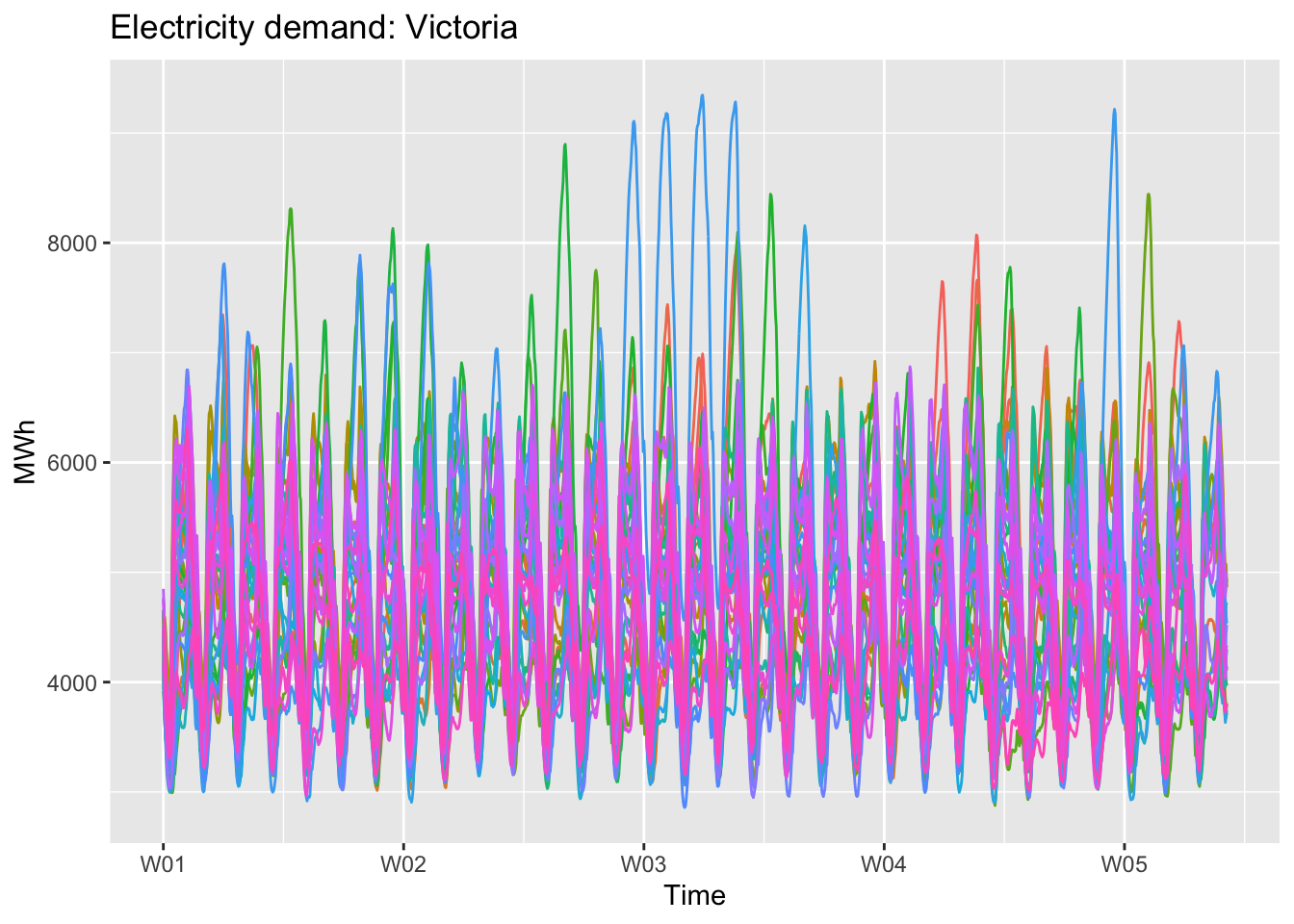

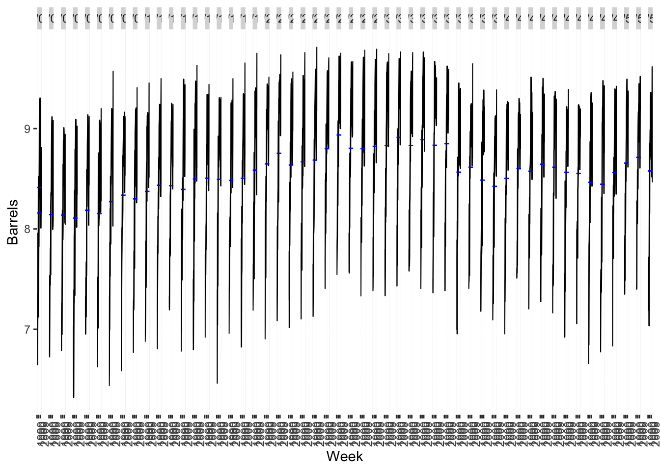
2.5 Seasonal subseries plots

The source of the section

Mini plots per each season.

a10 |>
  gg_subseries(Cost) +
  labs(y = '$ (millions)',
       title = 'Australian antidiabetic drug sales')

This plot is useful to identify changing within particular seasons.

2.5.1 Example: Australian holiday tourism

holidays <- tourism |>
  filter(Purpose == 'Holiday') |>
  group_by(State) |>
  summarise(Trips = sum(Trips))

holidays

## # A tsibble: 640 x 3 [1Q]
## # Key:       State [8]
##    State Quarter Trips
##    <chr>   <qtr> <dbl>
##  1 ACT   1998 Q1  196.
##  2 ACT   1998 Q2  127.
##  3 ACT   1998 Q3  111.
##  4 ACT   1998 Q4  170.
##  5 ACT   1999 Q1  108.
##  6 ACT   1999 Q2  125.
##  7 ACT   1999 Q3  178.
##  8 ACT   1999 Q4  218.
##  9 ACT   2000 Q1  158.
## 10 ACT   2000 Q2  155.
## # ℹ 630 more rows

Time plots of each series show that there is strong seasonality for most states, but that the seasonal peaks do not coincide.

holidays |>
  autoplot(Trips) +
  labs(y = 'Obernight trips (K)',
       title = 'Australian domestic holidays')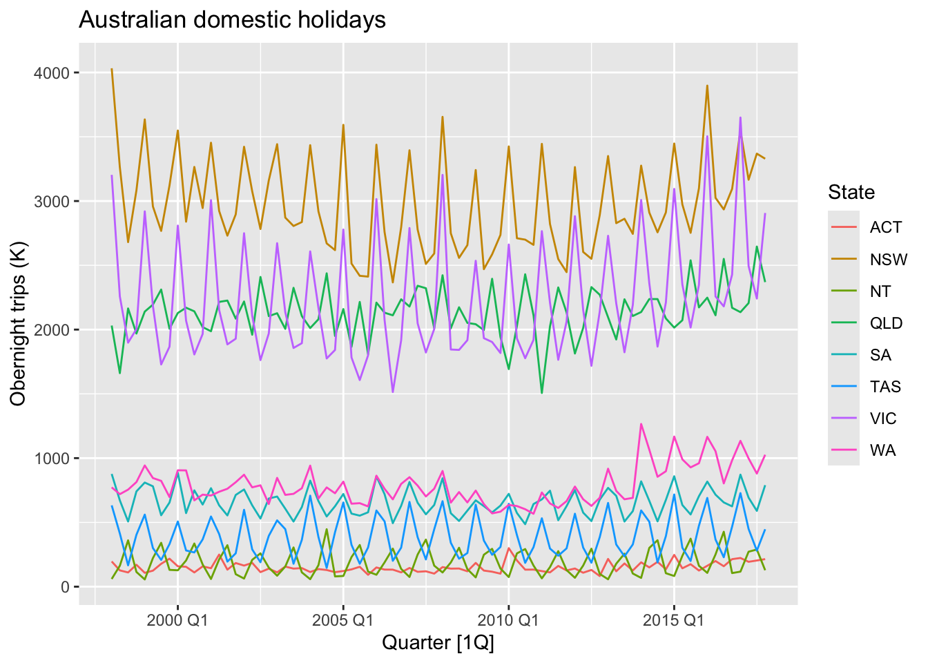

holidays |>
  gg_season(Trips) +
  labs(y = 'Obernight trips (K)',
       title = 'Australian domestic holidays')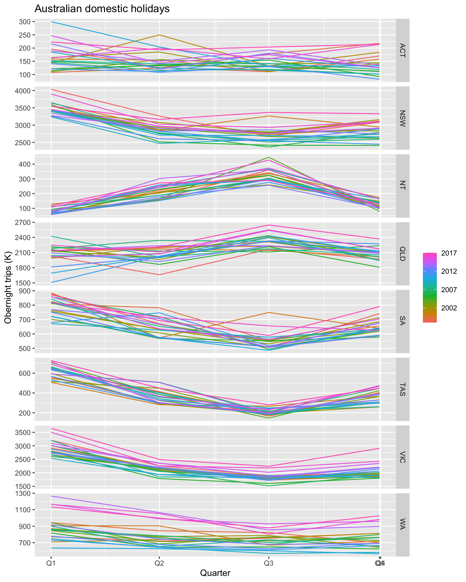

Subseries plot.

holidays |>
  gg_subseries(Trips) +
    labs(y = 'Obernight trips (K)',
       title = 'Australian domestic holidays')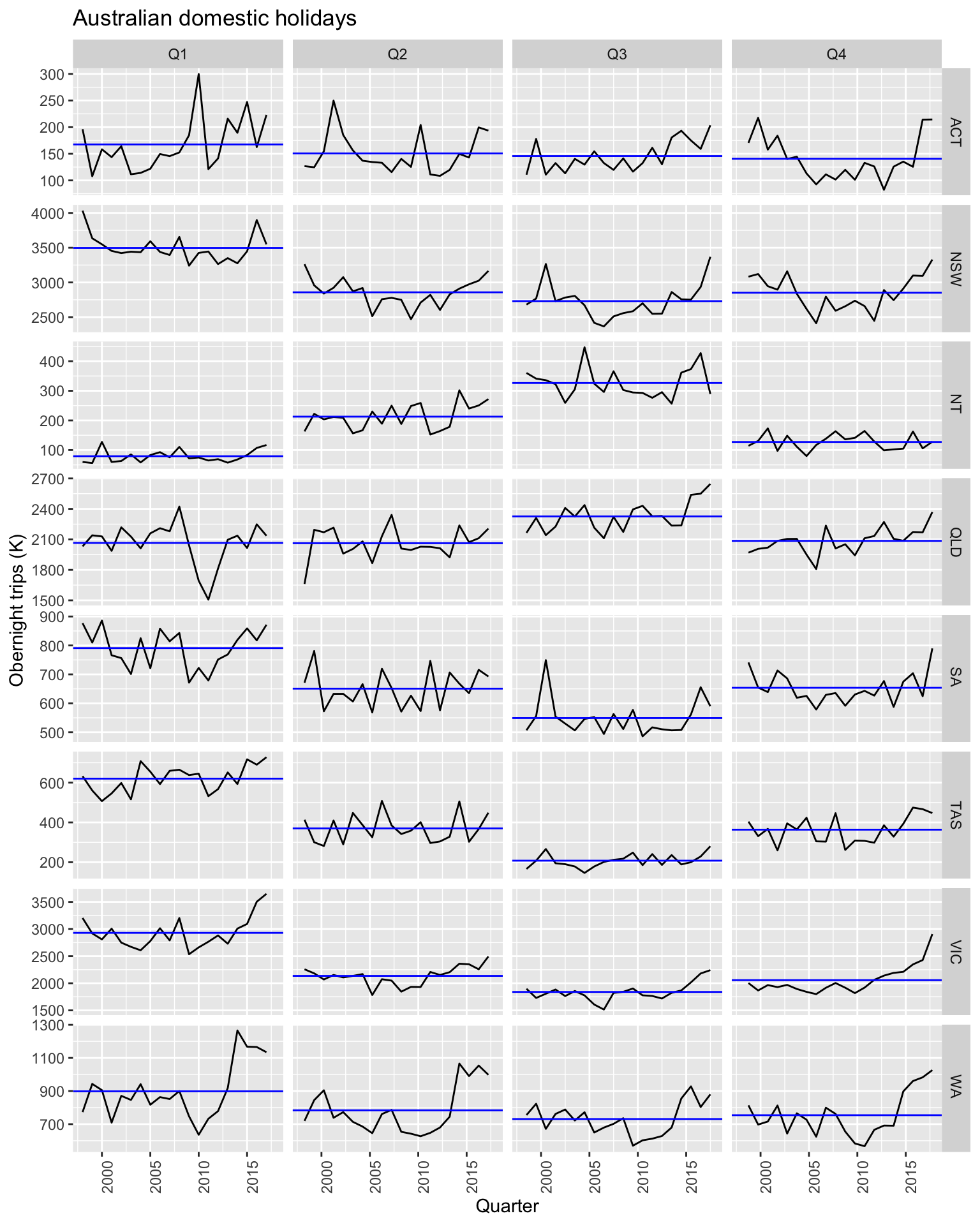

2.6 Scatterplots

The source of the section

Scatterplots are useful to explore relationship between time series.

vic_elec_day_type = vic_elec |>
  filter(year(Time) == 2014) |>
  mutate(Day_Type =  case_when(Holiday ~ "Holiday",
                               wday(Date) %in% 2:6 ~ "Weekday",
                               TRUE ~ "Weekend"))

vic_elec_day_type

## # A tsibble: 17,520 x 6 [30m] <Australia/Melbourne>
##    Time                Demand Temperature Date       Holiday Day_Type
##    <dttm>               <dbl>       <dbl> <date>     <lgl>   <chr>   
##  1 2014-01-01 00:00:00  4092.        18.7 2014-01-01 TRUE    Holiday 
##  2 2014-01-01 00:30:00  4198.        18.1 2014-01-01 TRUE    Holiday 
##  3 2014-01-01 01:00:00  3915.        18.2 2014-01-01 TRUE    Holiday 
##  4 2014-01-01 01:30:00  3673.        17.9 2014-01-01 TRUE    Holiday 
##  5 2014-01-01 02:00:00  3498.        17.6 2014-01-01 TRUE    Holiday 
##  6 2014-01-01 02:30:00  3339.        16.8 2014-01-01 TRUE    Holiday 
##  7 2014-01-01 03:00:00  3204.        16.3 2014-01-01 TRUE    Holiday 
##  8 2014-01-01 03:30:00  3100.        16.6 2014-01-01 TRUE    Holiday 
##  9 2014-01-01 04:00:00  3039.        16.6 2014-01-01 TRUE    Holiday 
## 10 2014-01-01 04:30:00  3012.        16.7 2014-01-01 TRUE    Holiday 
## # ℹ 17,510 more rows

vic_elec_day_type |>
  autoplot(facets=TRUE) +
  labs(y = "GWh",
       title = "Half-hourly electricity demand: Victoria")

## Plot variable not specified, automatically selected `.vars = Demand`

## Warning in geom_line(...): Ignoring unknown parameters: `facets`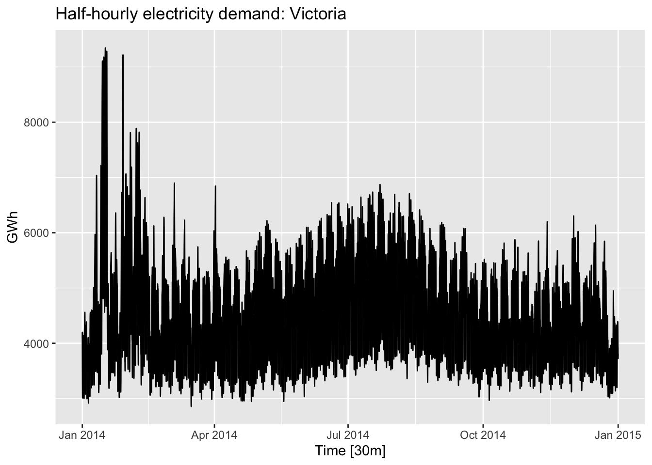

vic_elec_day_type |>
  autoplot(Temperature) +
  labs(y = "Degrees Celsius",
    title = "Half-hourly temperatures: Melbourne, Australia")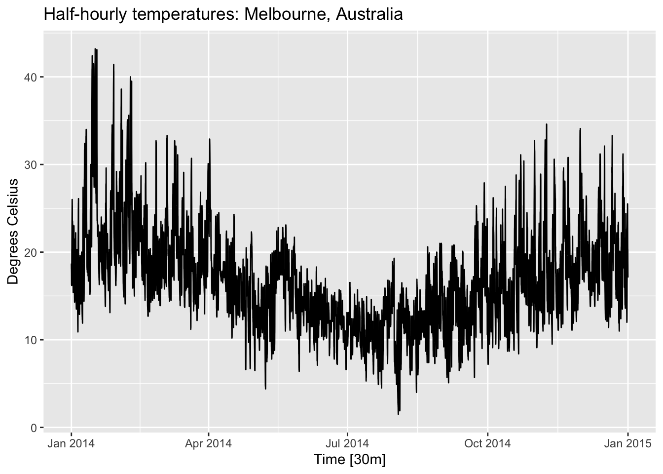

The relationship between demand and temperature.

vic_elec_day_type |>
  ggplot(aes(x = Temperature, y = Demand)) +
  geom_point() +
  labs(x = 'Temperature (Cº)',
       title = 'Electricity demand (GWh')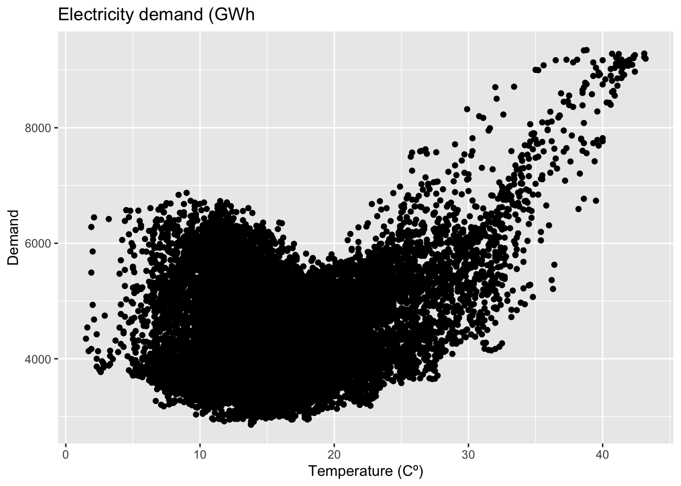

By the type of a day.

vic_elec_day_type |>
  ggplot(aes(x = Temperature, y = Demand, colour = Day_Type)) +
  geom_point() +
  labs(x = 'Temperature (Cº)',
       title = 'Electricity demand (GWh)')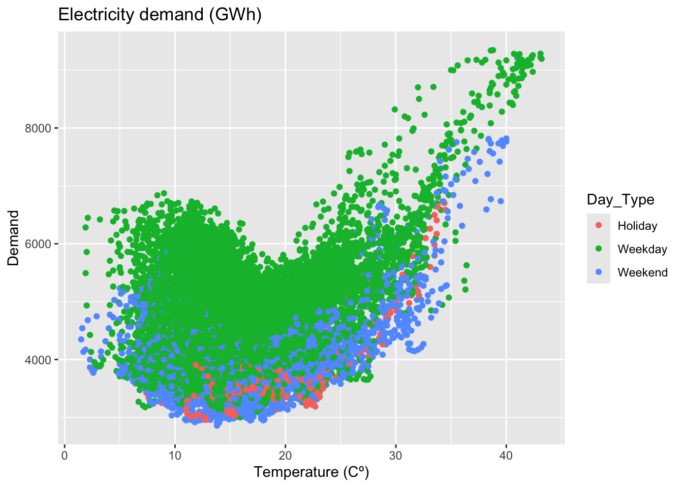

2.6.1 Correlation

The correlation coefficient.

\[ r = \frac {\sum{(x_t - \bar{x})(y_t - \bar{y})}}{\sqrt{\sum(x_t - \bar{x})^2}\sqrt{\sum(y_t - \bar{y})^2}}, -1 \leq r \leq 1 \]

2.6.2 Scatterplot matrices

tourism

## # A tsibble: 24,320 x 5 [1Q]
## # Key:       Region, State, Purpose [304]
##    Quarter Region   State Purpose  Trips
##      <qtr> <chr>    <chr> <chr>    <dbl>
##  1 1998 Q1 Adelaide SA    Business  135.
##  2 1998 Q2 Adelaide SA    Business  110.
##  3 1998 Q3 Adelaide SA    Business  166.
##  4 1998 Q4 Adelaide SA    Business  127.
##  5 1999 Q1 Adelaide SA    Business  137.
##  6 1999 Q2 Adelaide SA    Business  200.
##  7 1999 Q3 Adelaide SA    Business  169.
##  8 1999 Q4 Adelaide SA    Business  134.
##  9 2000 Q1 Adelaide SA    Business  154.
## 10 2000 Q2 Adelaide SA    Business  169.
## # ℹ 24,310 more rows

visitors <- tourism |>
  group_by(State) |>
  summarise(Trips = sum(Trips))

visitors

## # A tsibble: 640 x 3 [1Q]
## # Key:       State [8]
##    State Quarter Trips
##    <chr>   <qtr> <dbl>
##  1 ACT   1998 Q1  551.
##  2 ACT   1998 Q2  416.
##  3 ACT   1998 Q3  436.
##  4 ACT   1998 Q4  450.
##  5 ACT   1999 Q1  379.
##  6 ACT   1999 Q2  558.
##  7 ACT   1999 Q3  449.
##  8 ACT   1999 Q4  595.
##  9 ACT   2000 Q1  600.
## 10 ACT   2000 Q2  557.
## # ℹ 630 more rows

visitors |>
  ggplot(aes(x = Quarter, y = Trips)) +
  geom_line() +
  facet_grid(vars(State), scales = 'free_y') +
  labs(title = 'Australian domestic tourism',
       y = 'Overnight trips (K)')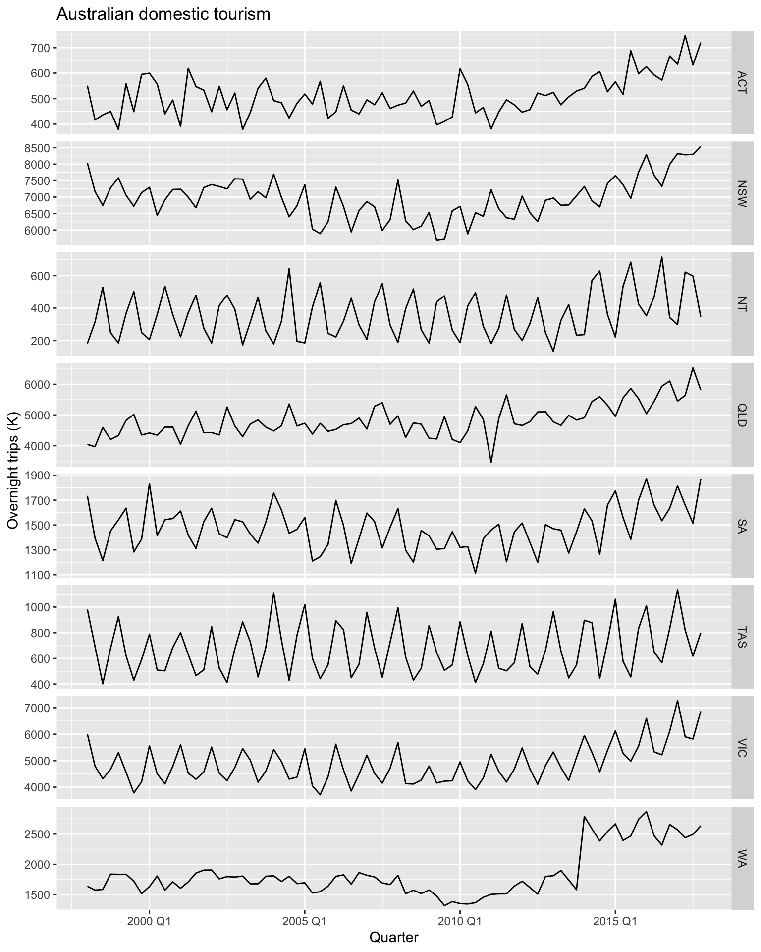

A scatterplot matrix displays the relationships between pairs of variables in a dataset by showing scatterplots for each combination of variables. This helps to visualize correlations, trends, and patterns between variables, making it easier to detect linear relationships, clusters, or outliers. Each scatterplot shows how one variable relates to another, and the diagonal typically contains the distribution (e.g., histograms, density) of each variable.

visitors |>
  pivot_wider(values_from = 'Trips', names_from = 'State') |>
  GGally::ggpairs(columns = 2:9)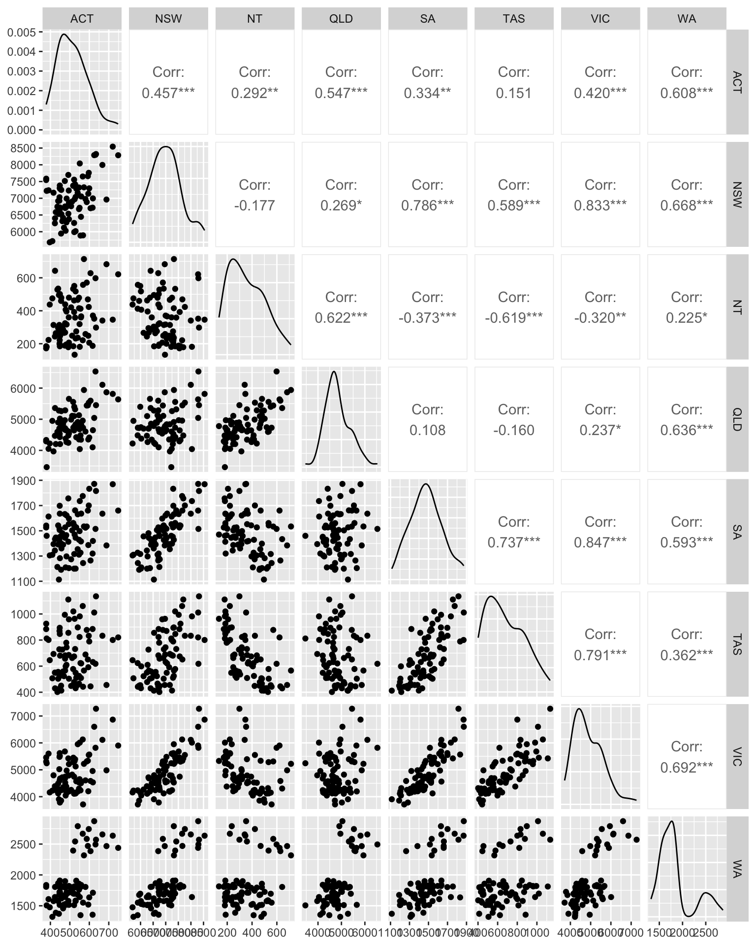

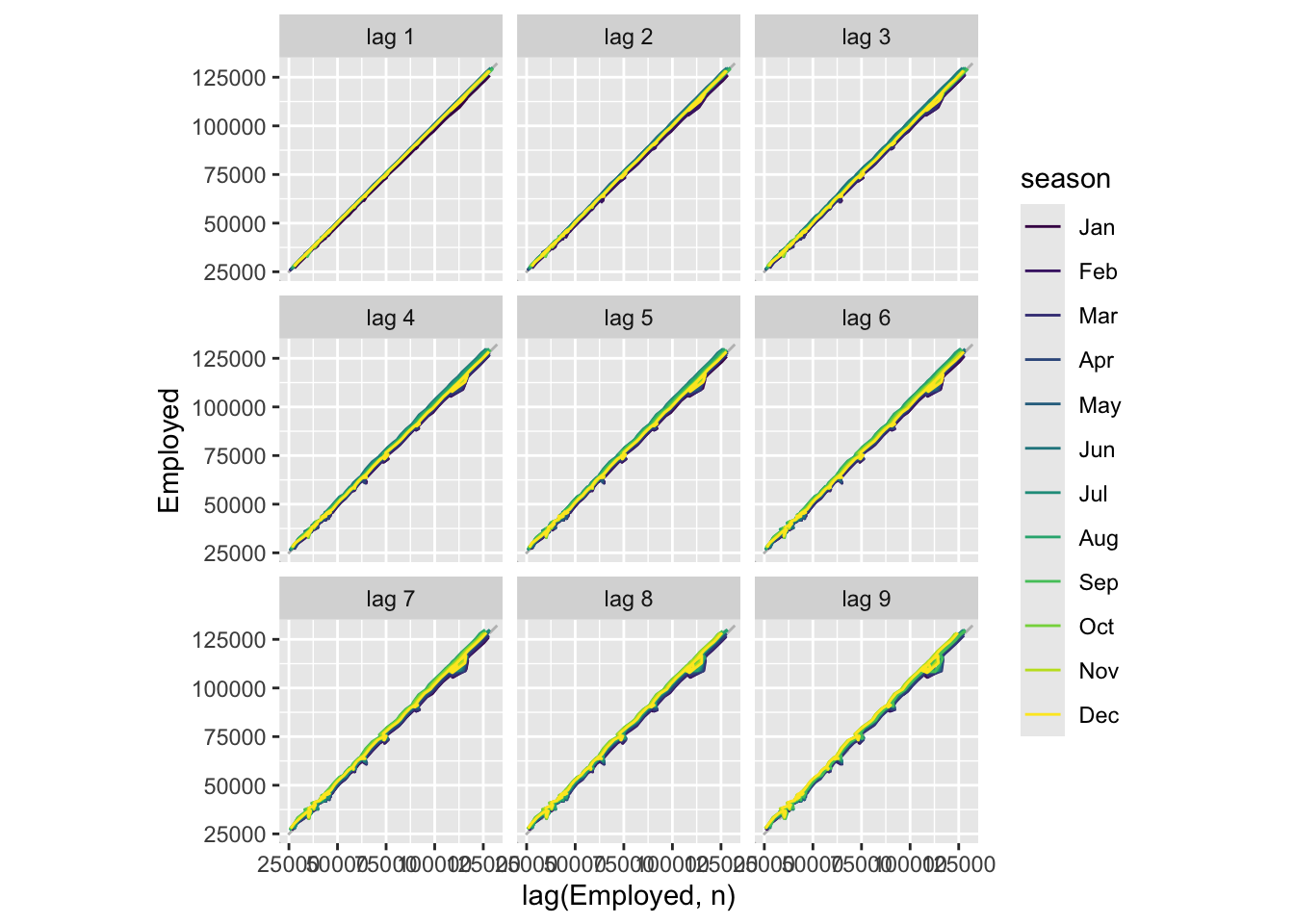
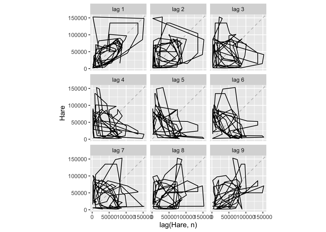
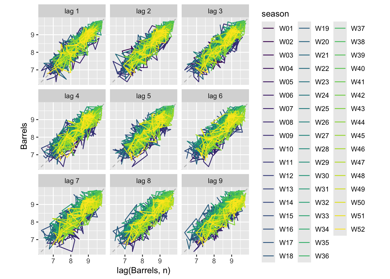
2.7 Lag plots

The source of the section

Lag plot uses to identify relationship between multiple time series.

new_production <- aus_production |>
  filter(year(Quarter) >= 1992)

new_production

## # A tsibble: 74 x 7 [1Q]
##    Quarter  Beer Tobacco Bricks Cement Electricity   Gas
##      <qtr> <dbl>   <dbl>  <dbl>  <dbl>       <dbl> <dbl>
##  1 1992 Q1   443    5777    383   1289       38332   117
##  2 1992 Q2   410    5853    404   1501       39774   151
##  3 1992 Q3   420    6416    446   1539       42246   175
##  4 1992 Q4   532    5825    420   1568       38498   129
##  5 1993 Q1   433    5724    394   1450       39460   116
##  6 1993 Q2   421    6036    462   1668       41356   149
##  7 1993 Q3   410    6570    475   1648       42949   163
##  8 1993 Q4   512    5675    443   1863       40974   138
##  9 1994 Q1   449    5311    421   1468       40162   127
## 10 1994 Q2   381    5717    475   1755       41199   159
## # ℹ 64 more rows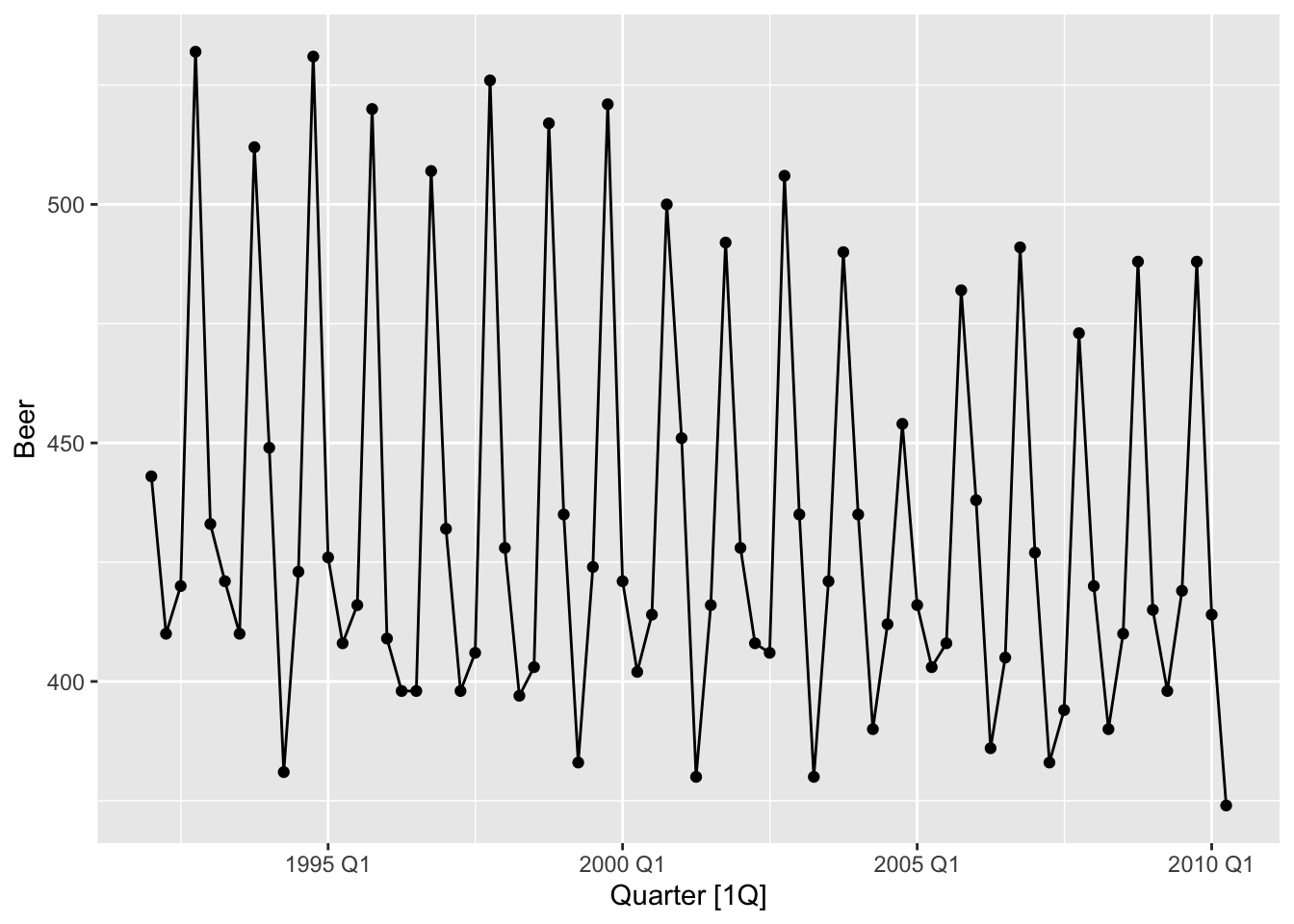

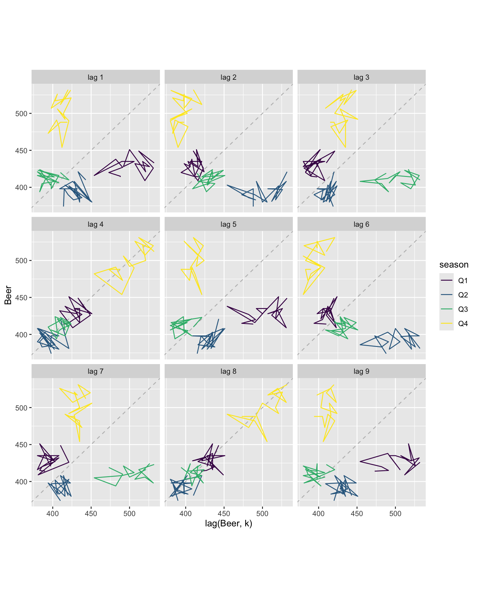
new_production |>
  autoplot(Beer) +
  geom_point()

Each graph shows \(y_t\) plotted against \(y_{t−k}\) for different values of \(k\).

new_production |>
  gg_lag(Beer, geom='point') +
  labs(x = 'lag(Beer, k)')

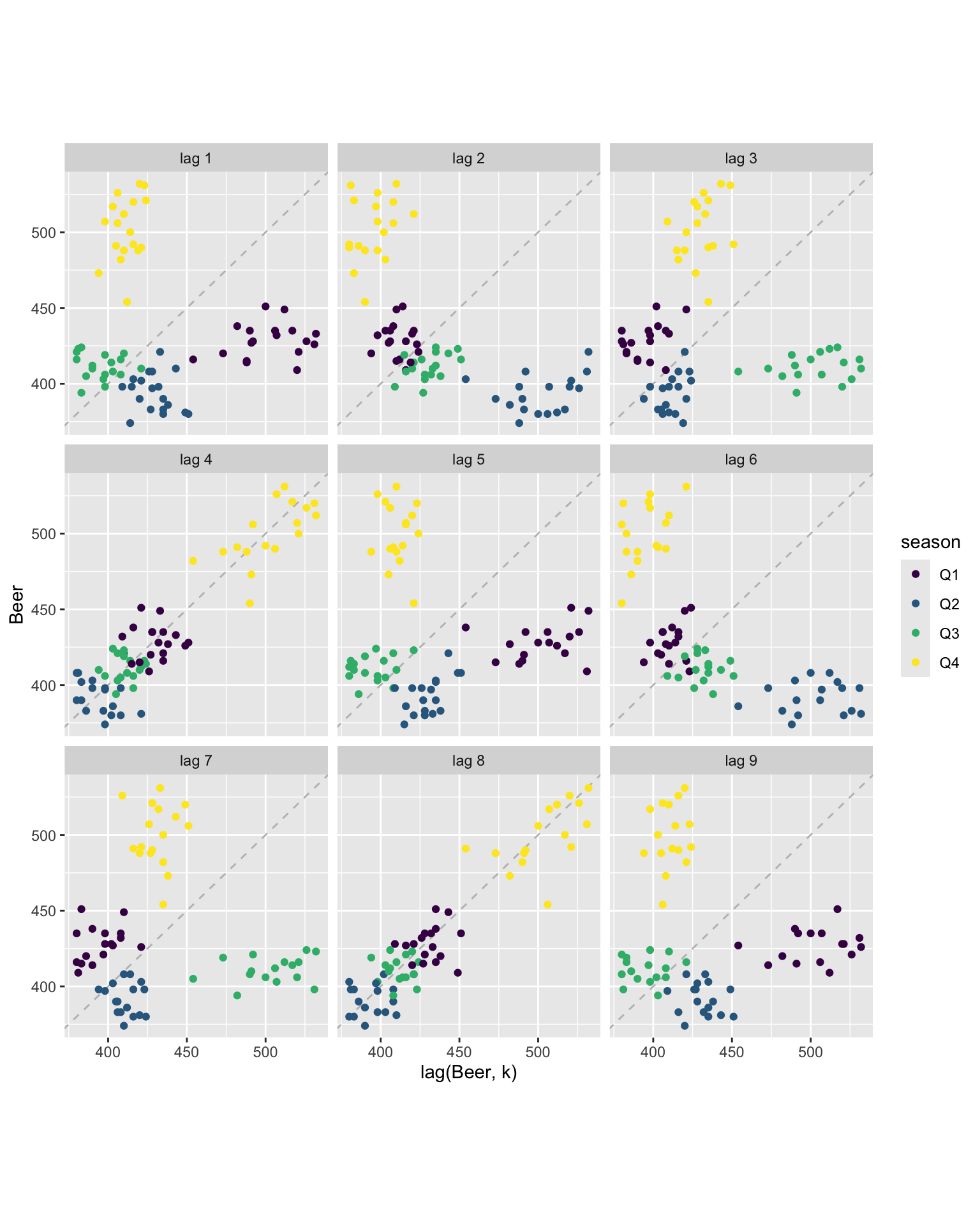
The relationship is strongly positive at lags 4 and 8, reflecting the strong seasonality in the data. The negative relationship seen for lags 2 and 6 occurs because peaks (in Q4) are plotted against troughs (in Q2)

new_production |>
  gg_lag(Beer, geom='path') +
  labs(x = 'lag(Beer, k)')

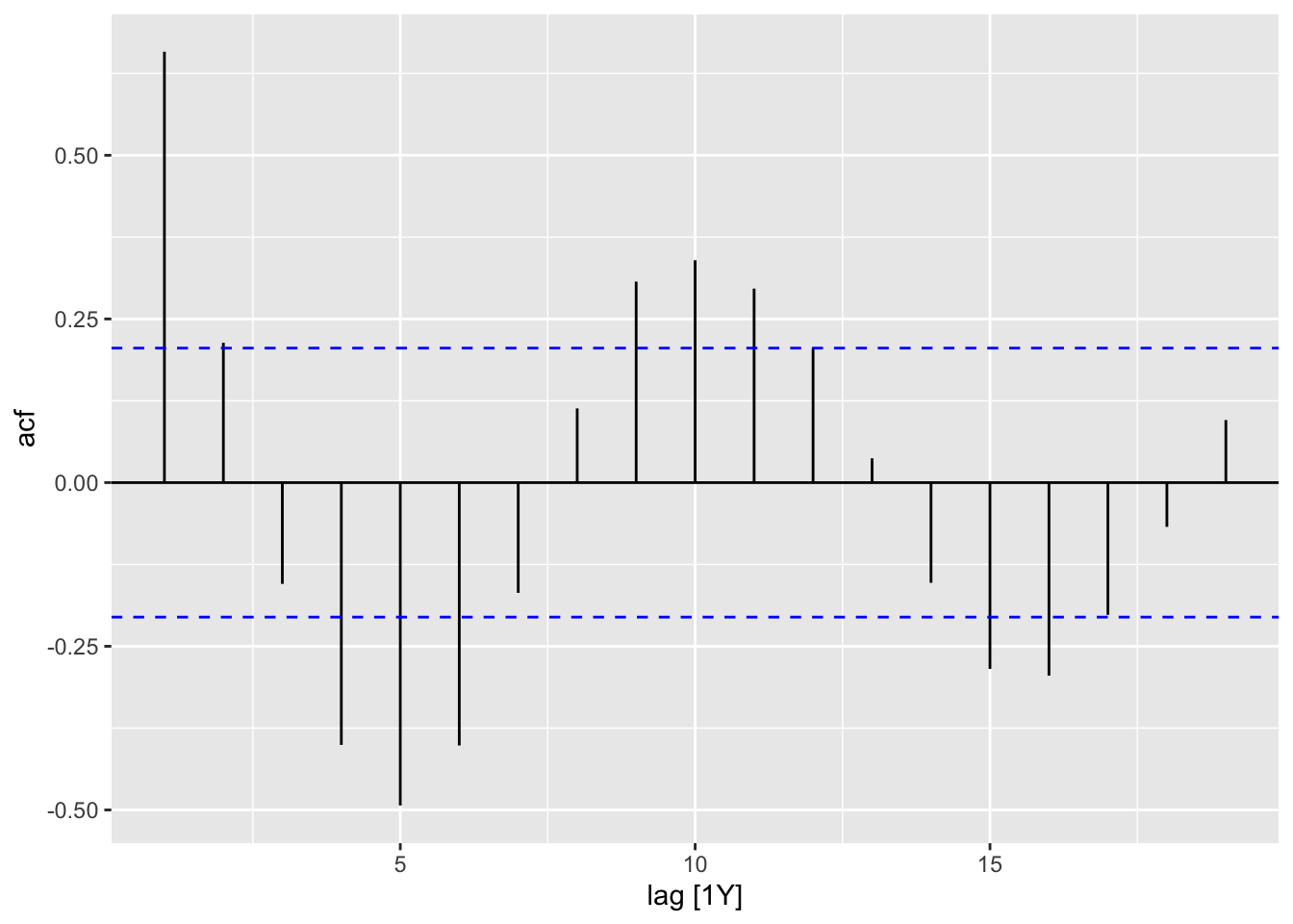
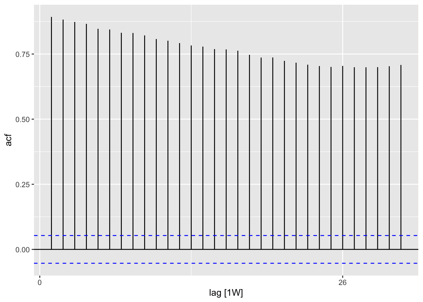
2.8 Autocorrelation

The source of the section

Autocorrelation measures the linear relationship between lagged values of a time series.

For example, \(r_1\) measures the relationship between \(y_t\) and \(y_{t−1}\), \(r_2\) measures the relationship between \(y_t\) and $y_{t−2}, and so on.

\[ ACF_1 = r_1 = Corr(y_t, y_{t-1}) \\ ACF_2 = r_2 = Corr(y_t, y_{t-2}) \\ ... \\ ACF_k = r_k = Corr(y_t, y_{t-k}) \]

The value of \(r_k\) can be written as

$$

r_k = {_{t=1}^T (y_t - {y})^2}

$$

where \(T\) is the length of the time series. The autocorrelation coefficients make up the autocorrelation function or ACF.

new_production |>
  ACF(Beer, lag_max = 9)

## # A tsibble: 9 x 2 [1Q]
##        lag     acf
##   <cf_lag>   <dbl>
## 1       1Q -0.102 
## 2       2Q -0.657 
## 3       3Q -0.0603
## 4       4Q  0.869 
## 5       5Q -0.0892
## 6       6Q -0.635 
## 7       7Q -0.0542
## 8       8Q  0.832 
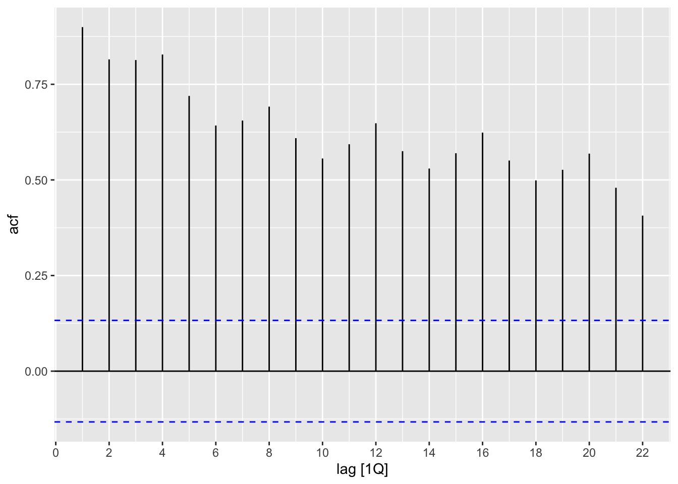
## 9       9Q -0.108

Build correlogram.

new_production |>
  ACF(Beer) |>
  autoplot() + labs(title="Australian beer production")

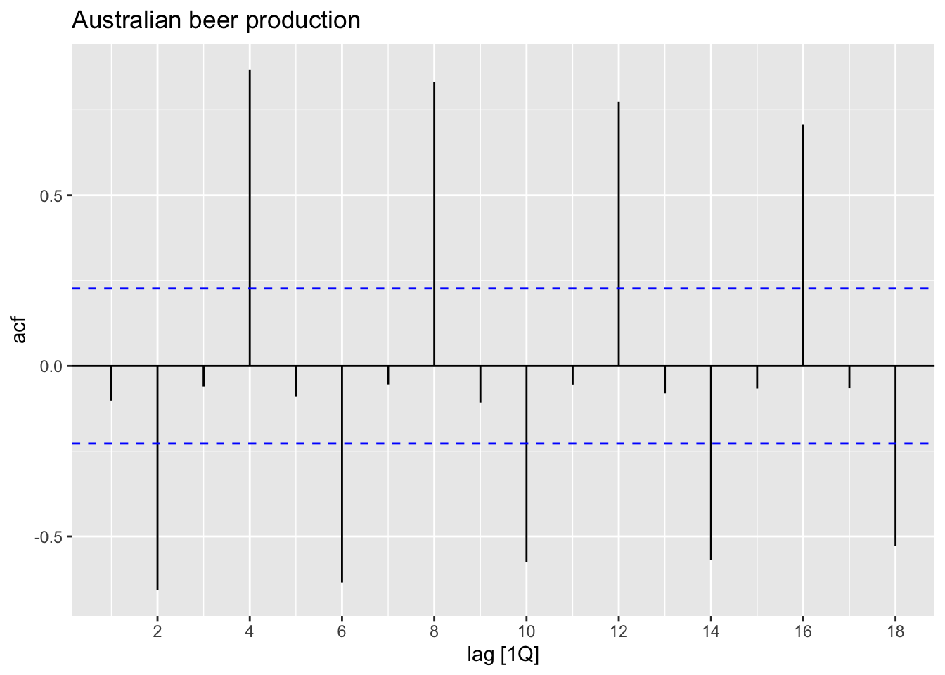
Interpretaion:

• \(r_4\) is higher than for the other lags. This is due to the seasonal pattern in the data: the peaks tend to be four quarters apart and the troughs tend to be four quarters apart.
• \(r_2\) is more negative than for the other lags because troughs tend to be two quarters behind peaks.
• The dashed blue lines indicate whether the correlations are significantly different from zero.

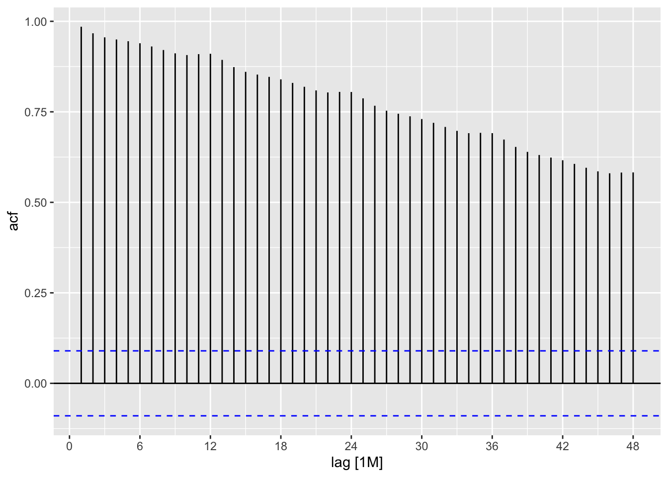
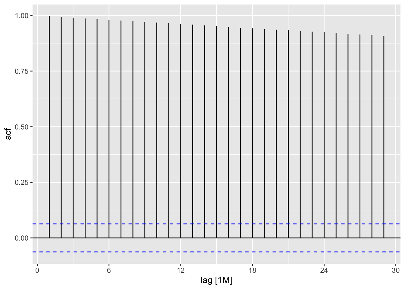
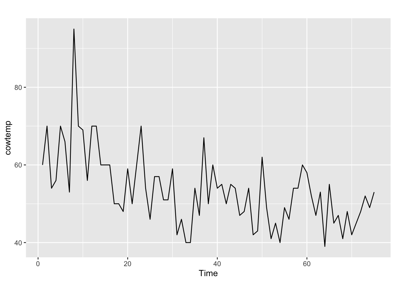
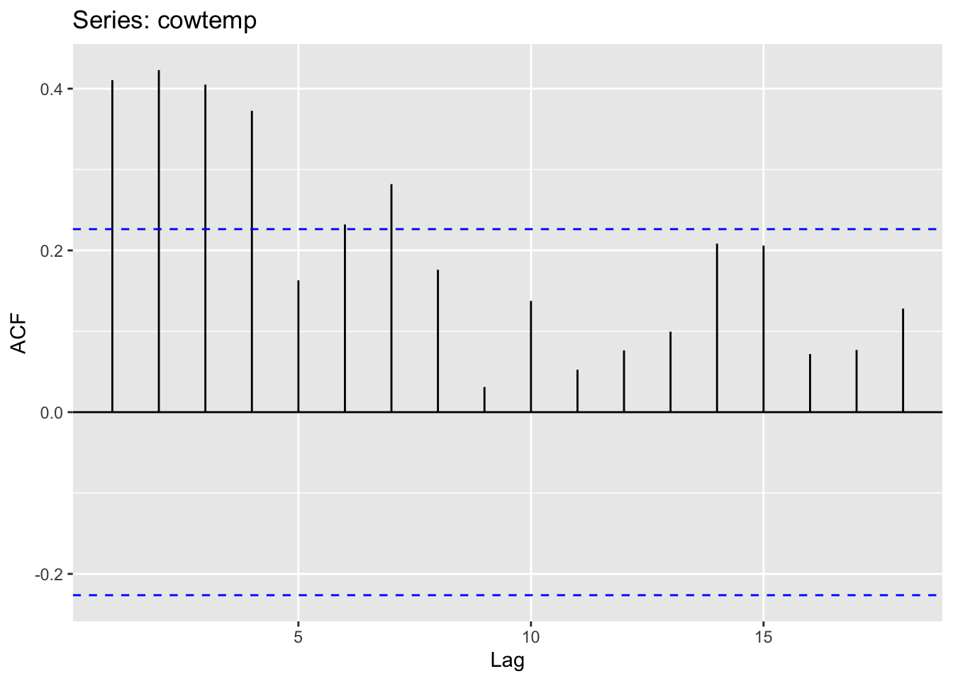
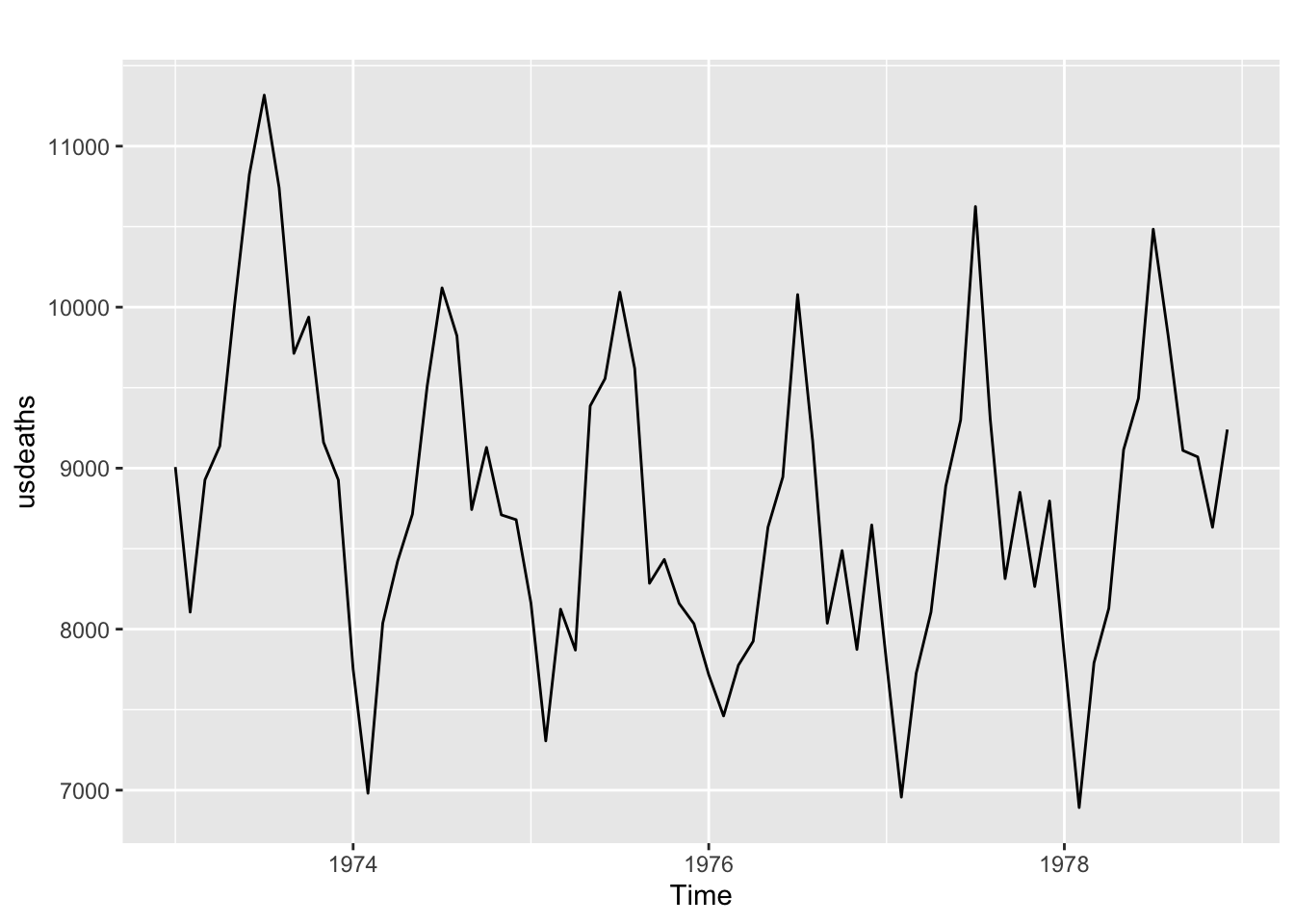
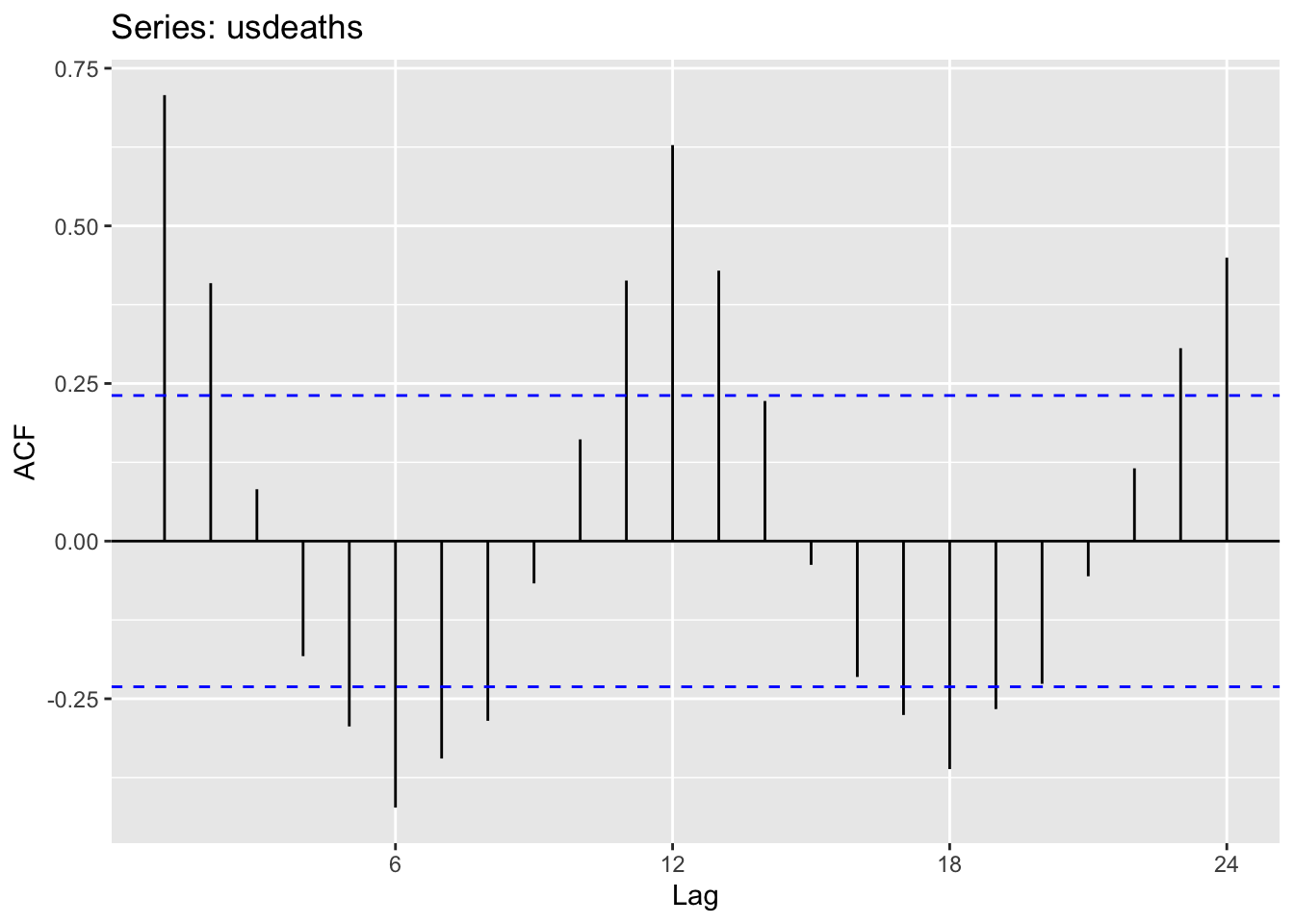
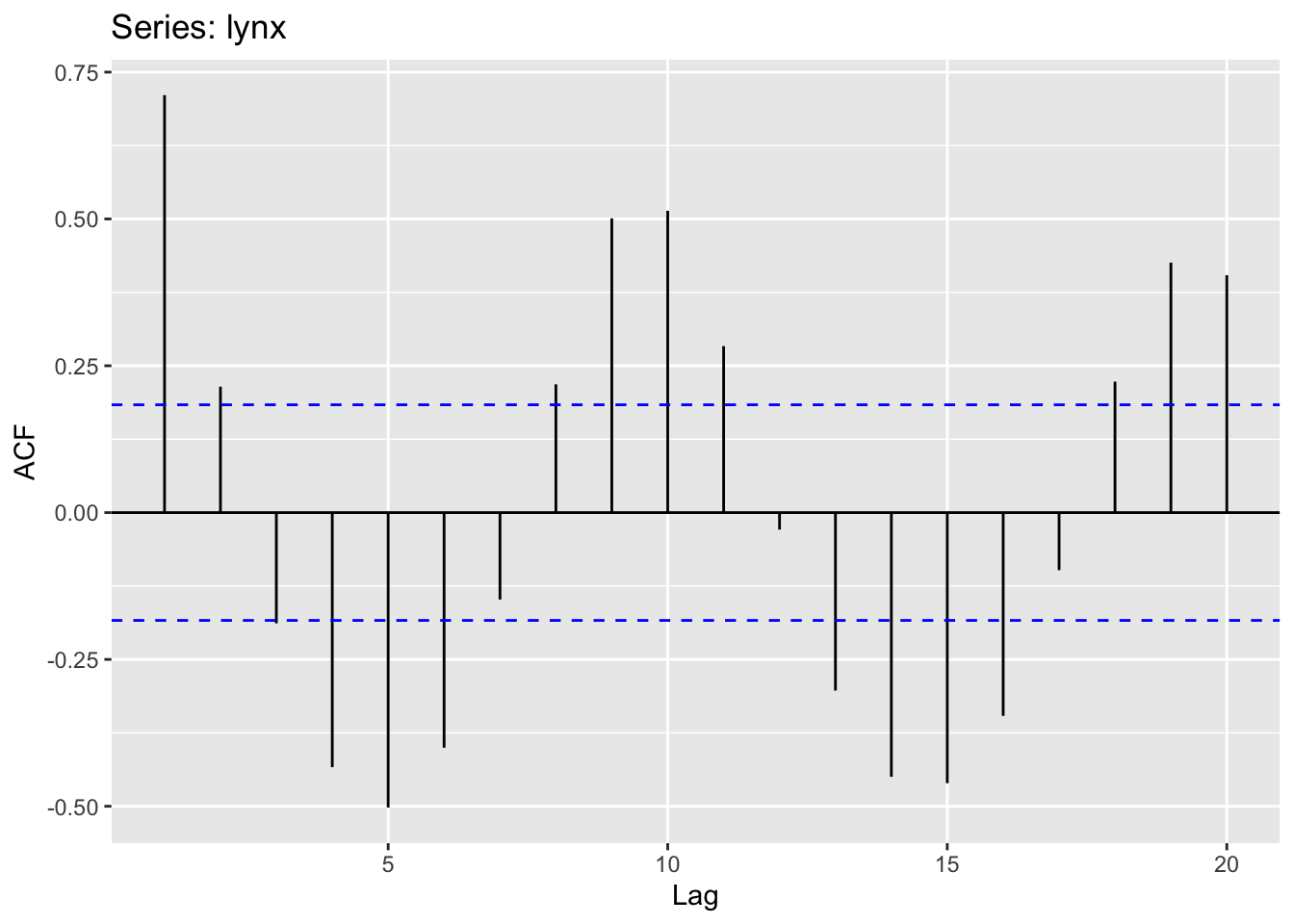
2.8.1 Trend and seasonality in ACF plots

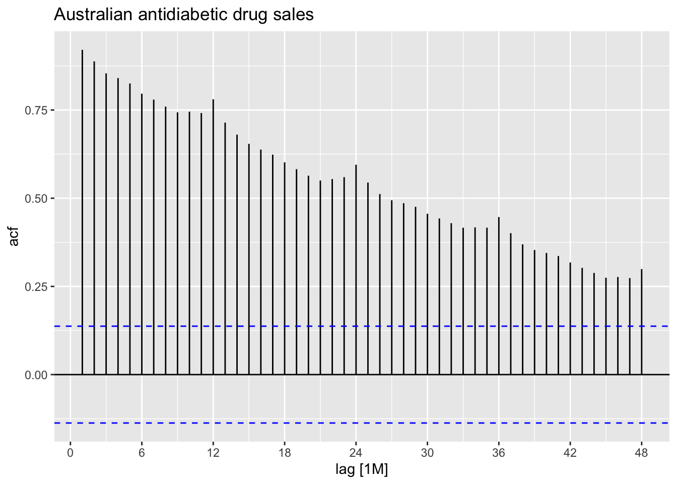
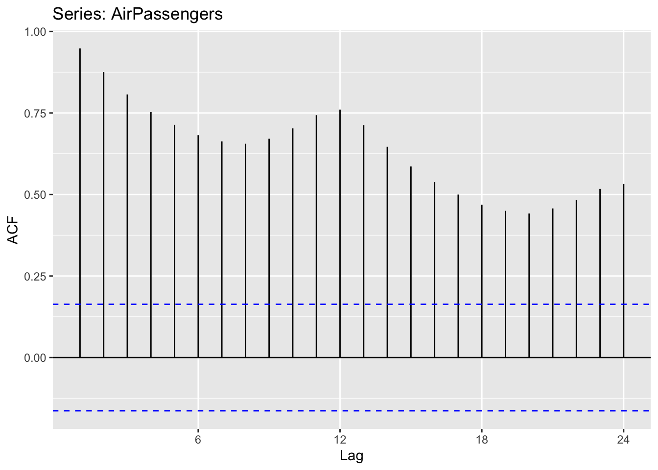
Trend: Indicated by a slow decay in autocorrelations over increasing lags, suggesting a persistent pattern. ACF values decrease gradually without sharp drops.

Seasonality: Shown by regular spikes at consistent intervals (lags), reflecting repeating cycles. For example, monthly data with yearly seasonality will spike at lag 12, 24, etc.

When data are both trended and seasonal, you see a combination of these effects.

a10 |>
  ACF(Cost, lag_max = 48) |>
  autoplot() +
  labs(title = 'Australian antidiabetic drug sales')

retail <- us_employment |>
  filter(Title == 'Retail Trade', year(Month) >= 1980) 

retail |>
  autoplot(Employed)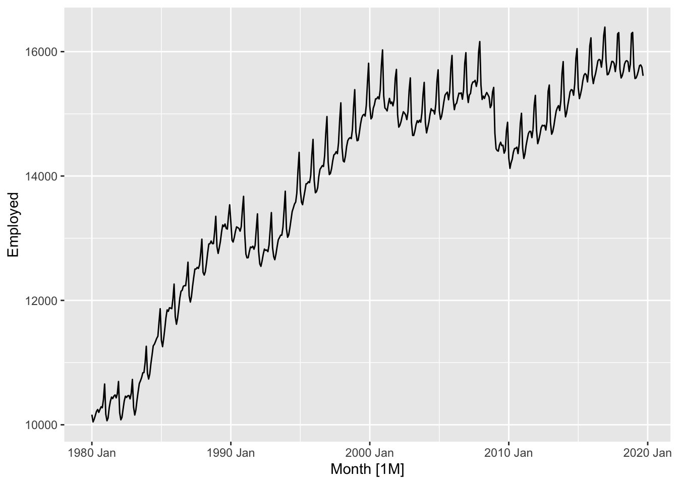

retail |>
  ACF(Employed, lag_max = 48) |>
  autoplot()

google_2015 <- gafa_stock |>
  filter(Symbol == 'GOOG', year(Date) == 2015) |>
  select(Date, Close)

google_2015

## # A tsibble: 252 x 2 [!]
##    Date       Close
##    <date>     <dbl>
##  1 2015-01-02  522.
##  2 2015-01-05  511.
##  3 2015-01-06  499.
##  4 2015-01-07  498.
##  5 2015-01-08  500.
##  6 2015-01-09  493.
##  7 2015-01-12  490.
##  8 2015-01-13  493.
##  9 2015-01-14  498.
## 10 2015-01-15  499.
## # ℹ 242 more rows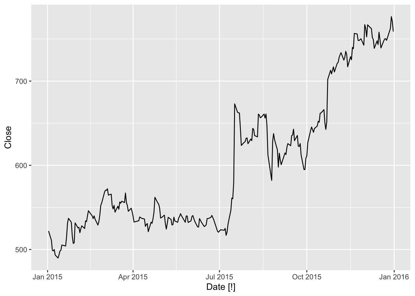

google_2015 |>
  autoplot(Close)

google_2015 |>
  ACF(Close, lag_max = 100) |>
  autoplot()

## Warning: Provided data has an irregular interval, results should be treated with caution. Computing ACF by observation.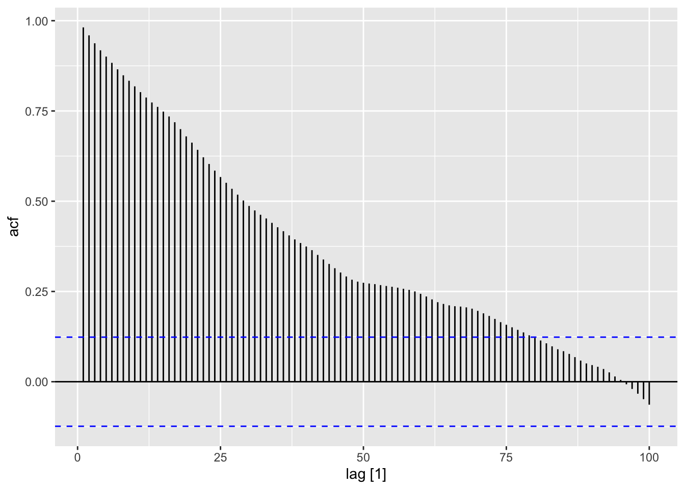

2.9 White moise

The source of the section

Time series that show no autocorrelation are called white noise.

set.seed(30)
y <- tsibble(sample = 1:50,
             wn = rnorm(50),
             index = sample)

y |> 
  autoplot(wn) +
  labs(title = 'White noise', y = '')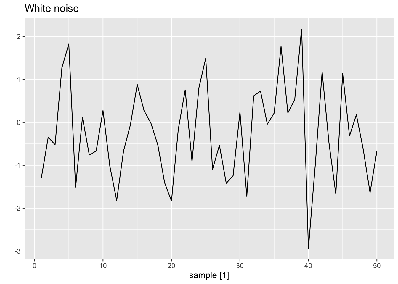

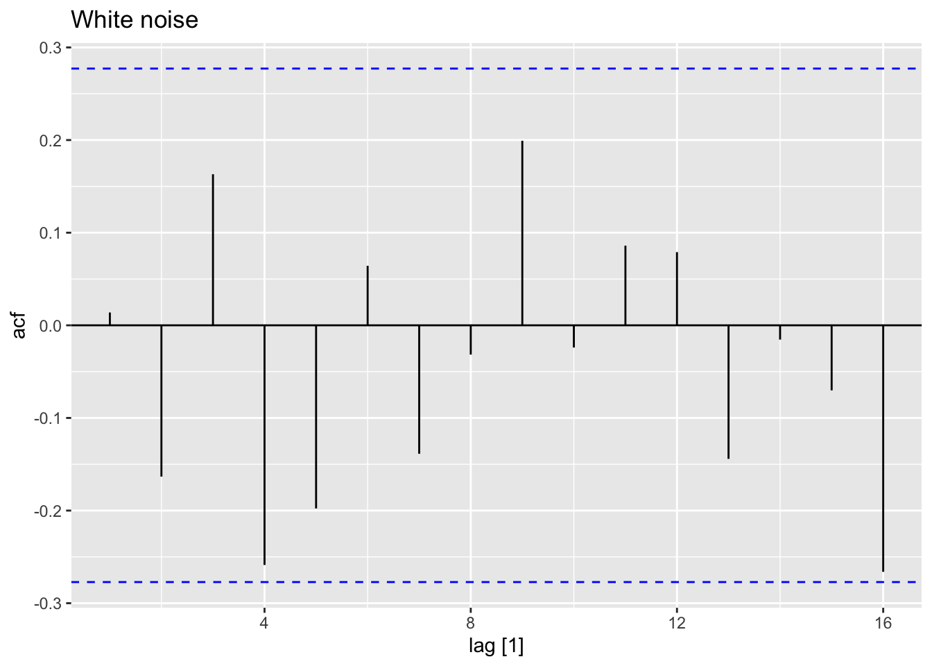
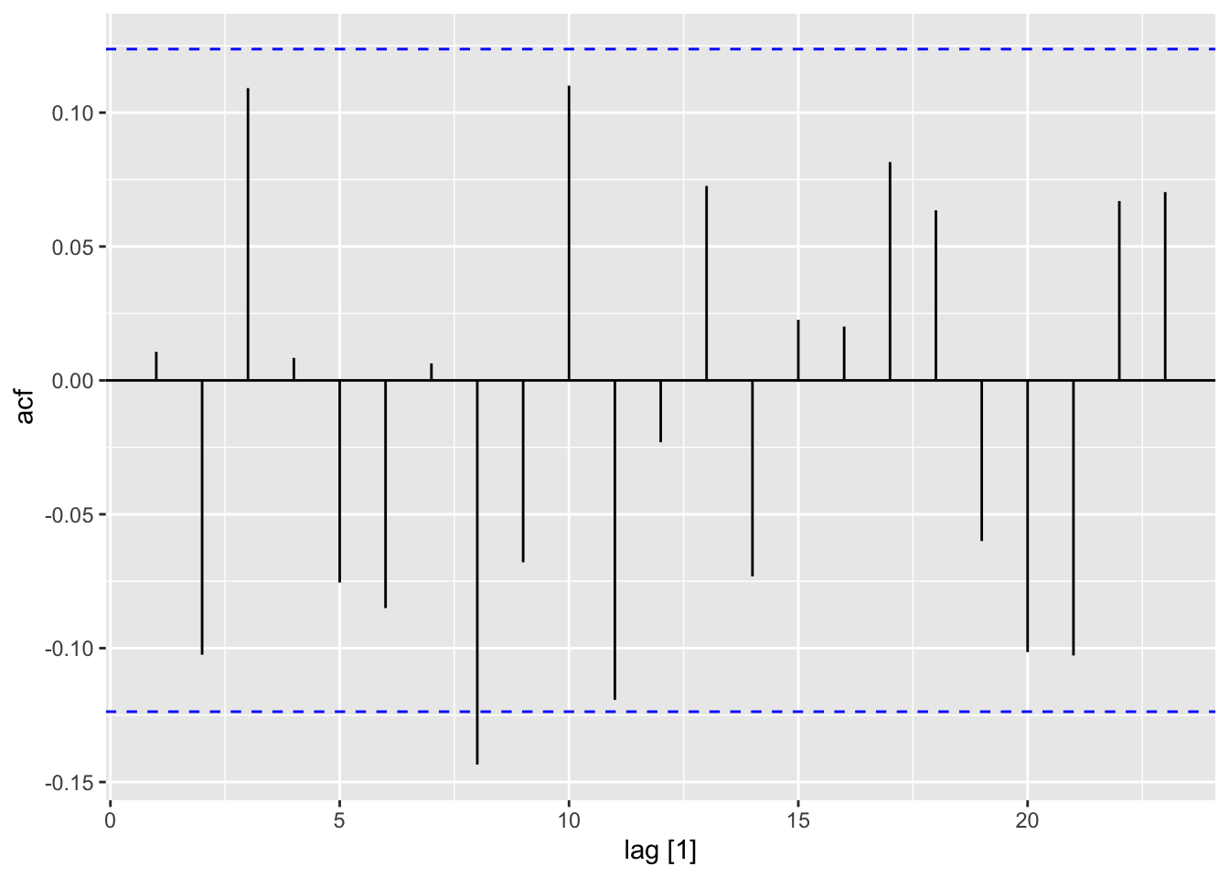
y |>
  ACF(wn) |>
  autoplot() +
  labs(title = 'White noise')

For white noise series, we expect each autocorrelation to be close to zero. For a white noise series, we expect 95% of the spikes in the ACF to lie within \(\pm 1.96/\sqrt{T}\), where \(T\) is the length of the time series.

If one or more large spikes are outside these bounds, or if substantially more than 5% of spikes are outside these bounds, then the series is probably not white noise.

2.10 Excercises

• Bricks from aus_production

?aus_production
# Quarterly estimates of selected indicators of manufacturing production in Australia.
# Bricks:   Clay brick production in millions of bricks.

aus_production

## # A tsibble: 218 x 7 [1Q]
##    Quarter  Beer Tobacco Bricks Cement Electricity   Gas
##      <qtr> <dbl>   <dbl>  <dbl>  <dbl>       <dbl> <dbl>
##  1 1956 Q1   284    5225    189    465        3923     5
##  2 1956 Q2   213    5178    204    532        4436     6
##  3 1956 Q3   227    5297    208    561        4806     7
##  4 1956 Q4   308    5681    197    570        4418     6
##  5 1957 Q1   262    5577    187    529        4339     5
##  6 1957 Q2   228    5651    214    604        4811     7
##  7 1957 Q3   236    5317    227    603        5259     7
##  8 1957 Q4   320    6152    222    582        4735     6
##  9 1958 Q1   272    5758    199    554        4608     5
## 10 1958 Q2   233    5641    229    620        5196     7
## # ℹ 208 more rows

# What is the time interval: Quarter

aus_production |>
  autoplot(Bricks) +
  labs(y = 'Bricks (million)', title = 'Quarterly production of bricks (million) in Australia')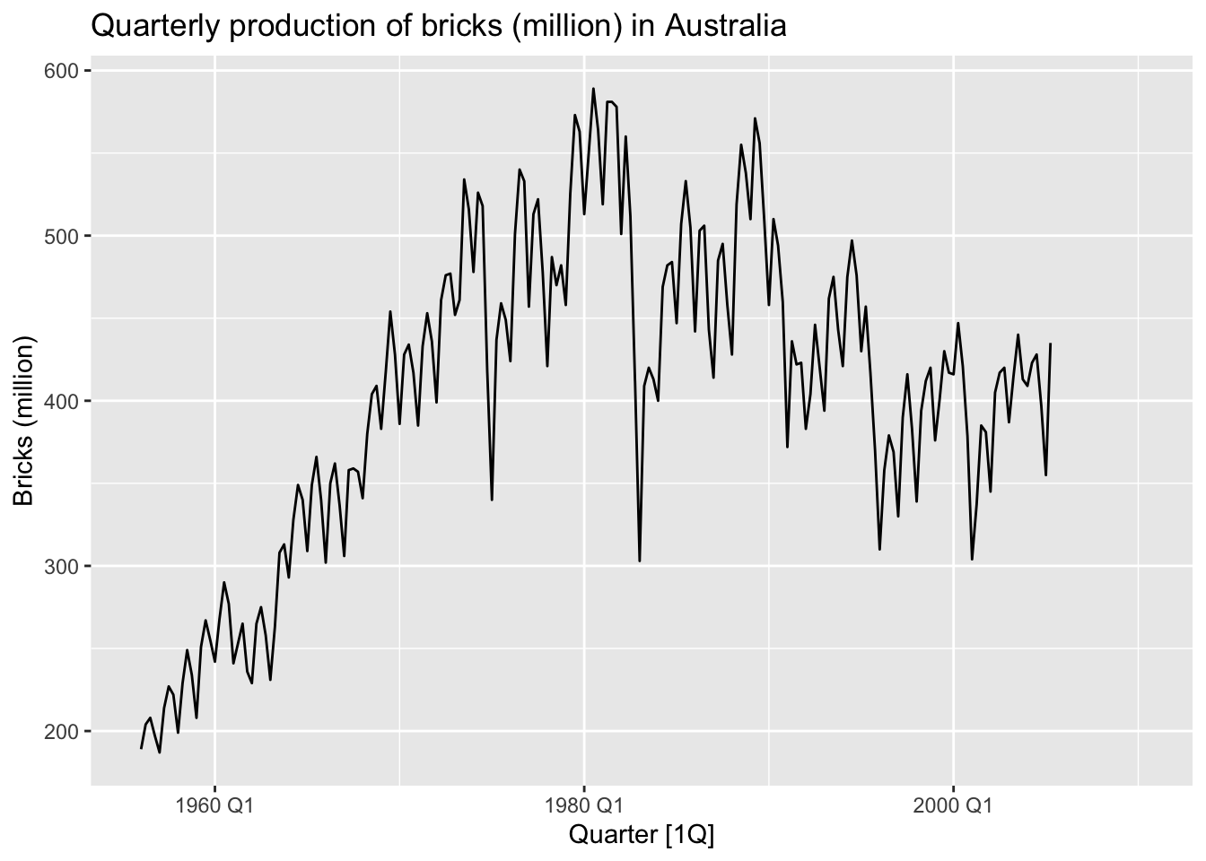

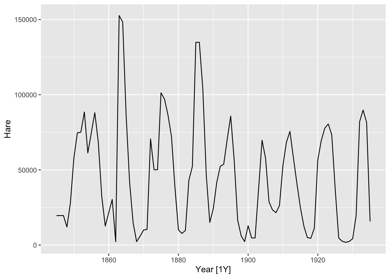
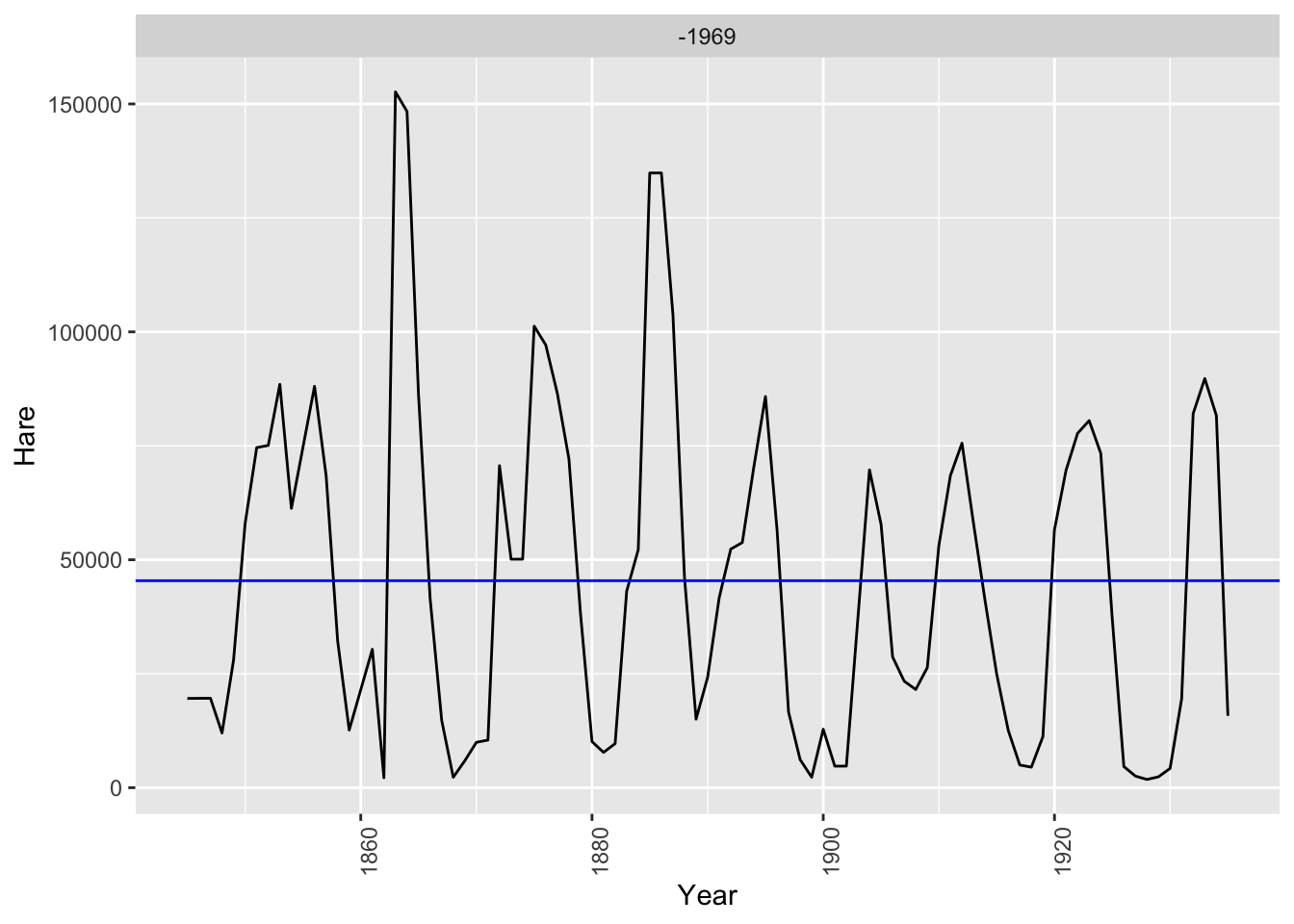
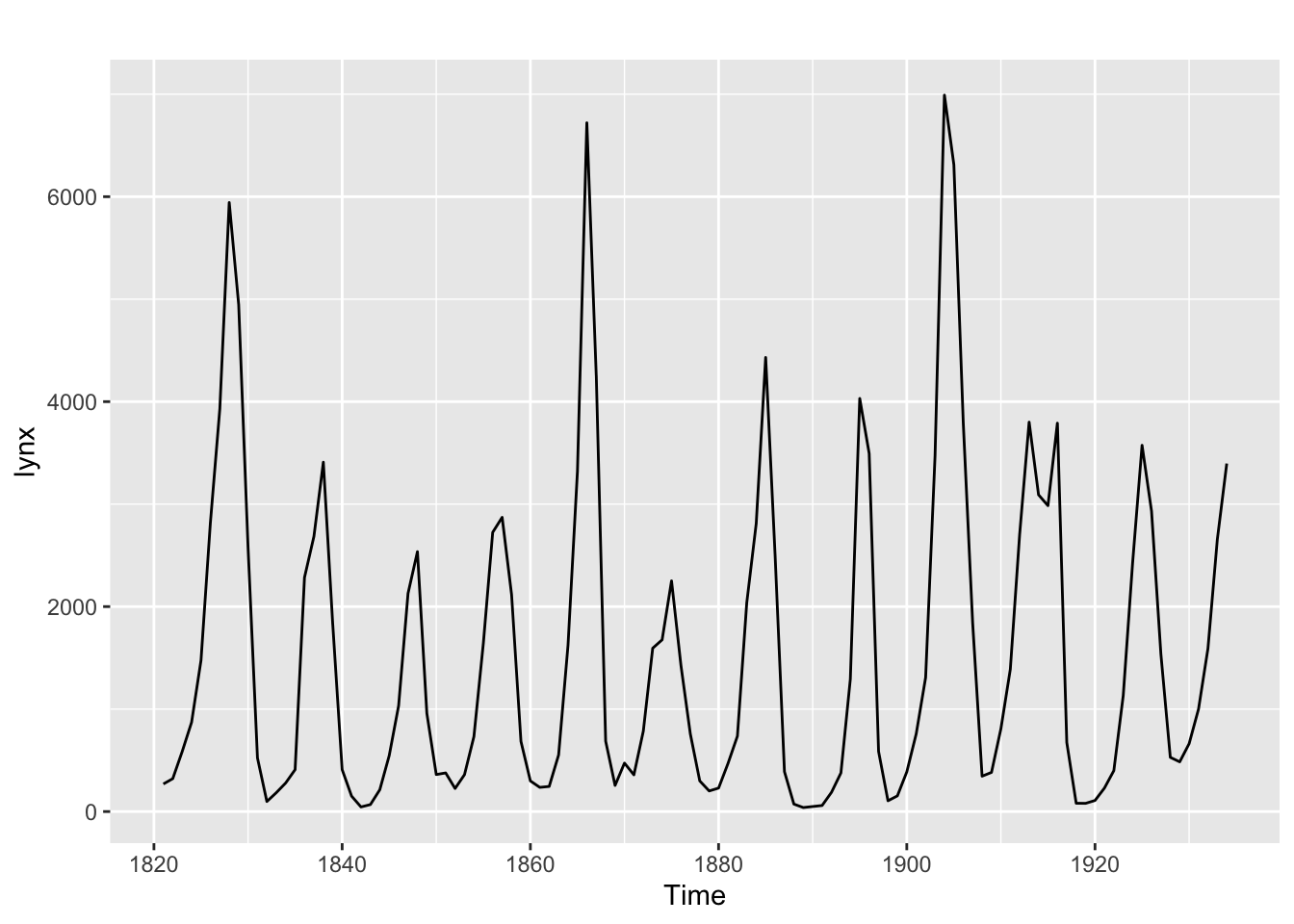
• Lynx from pelt

?pelt
# Hudson Bay Company trading records for Snowshoe Hare and Canadian Lynx furs from 1845 to 1935. This data contains trade records for all areas of the company.
# Lynx: The number of Canadian Lynx pelts traded.

pelt

## # A tsibble: 91 x 3 [1Y]
##     Year  Hare  Lynx
##    <dbl> <dbl> <dbl>
##  1  1845 19580 30090
##  2  1846 19600 45150
##  3  1847 19610 49150
##  4  1848 11990 39520
##  5  1849 28040 21230
##  6  1850 58000  8420
##  7  1851 74600  5560
##  8  1852 75090  5080
##  9  1853 88480 10170
## 10  1854 61280 19600
## # ℹ 81 more rows

# What is the time interval: Year

pelt |>
  autoplot(Lynx) +
  labs(y = 'Number of Lynx', title = 'Annual trading of Lynx')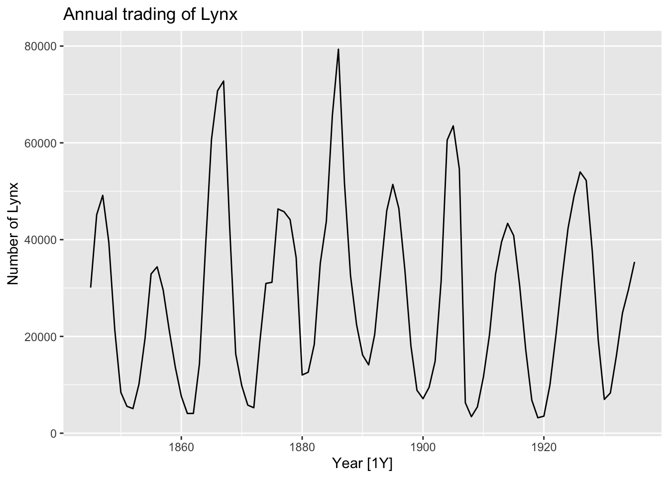

• Close from gafa_stock

?gafa_stock
# Historical stock prices from 2014-2018 for Google, Amazon, Facebook and Apple. All prices are in $USD.
# Close:    The closing price for the stock.

gafa_stock

## # A tsibble: 5,032 x 8 [!]
## # Key:       Symbol [4]
##    Symbol Date        Open  High   Low Close Adj_Close    Volume
##    <chr>  <date>     <dbl> <dbl> <dbl> <dbl>     <dbl>     <dbl>
##  1 AAPL   2014-01-02  79.4  79.6  78.9  79.0      67.0  58671200
##  2 AAPL   2014-01-03  79.0  79.1  77.2  77.3      65.5  98116900
##  3 AAPL   2014-01-06  76.8  78.1  76.2  77.7      65.9 103152700
##  4 AAPL   2014-01-07  77.8  78.0  76.8  77.1      65.4  79302300
##  5 AAPL   2014-01-08  77.0  77.9  77.0  77.6      65.8  64632400
##  6 AAPL   2014-01-09  78.1  78.1  76.5  76.6      65.0  69787200
##  7 AAPL   2014-01-10  77.1  77.3  75.9  76.1      64.5  76244000
##  8 AAPL   2014-01-13  75.7  77.5  75.7  76.5      64.9  94623200
##  9 AAPL   2014-01-14  76.9  78.1  76.8  78.1      66.1  83140400
## 10 AAPL   2014-01-15  79.1  80.0  78.8  79.6      67.5  97909700
## # ℹ 5,022 more rows

# What is the time interval: Trading days

gafa_stock |>
  autoplot(Close) +
  facet_grid(vars(Symbol), scale = 'free_y') +
  labs(y = '$USD', title = 'Historical stock prices from 2014-2018',
       subtitle = 'Google, Amazon, Facebook and Apple')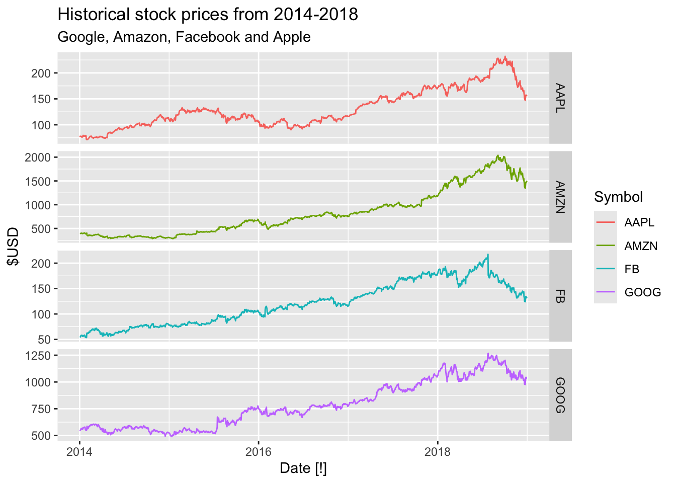

• Demand from vic_elec

?vic_elec
# vic_elec is a half-hourly tsibble with three values:
# Demand:   Total electricity demand in MWh.

vic_elec

## # A tsibble: 52,608 x 5 [30m] <Australia/Melbourne>
##    Time                Demand Temperature Date       Holiday
##    <dttm>               <dbl>       <dbl> <date>     <lgl>  
##  1 2012-01-01 00:00:00  4383.        21.4 2012-01-01 TRUE   
##  2 2012-01-01 00:30:00  4263.        21.0 2012-01-01 TRUE   
##  3 2012-01-01 01:00:00  4049.        20.7 2012-01-01 TRUE   
##  4 2012-01-01 01:30:00  3878.        20.6 2012-01-01 TRUE   
##  5 2012-01-01 02:00:00  4036.        20.4 2012-01-01 TRUE   
##  6 2012-01-01 02:30:00  3866.        20.2 2012-01-01 TRUE   
##  7 2012-01-01 03:00:00  3694.        20.1 2012-01-01 TRUE   
##  8 2012-01-01 03:30:00  3562.        19.6 2012-01-01 TRUE   
##  9 2012-01-01 04:00:00  3433.        19.1 2012-01-01 TRUE   
## 10 2012-01-01 04:30:00  3359.        19.0 2012-01-01 TRUE   
## # ℹ 52,598 more rows

# What is the time interval: 30 m

vic_elec |>
  autoplot(Demand) +
  labs(y = 'Demand (MWh)', title = 'Total electricity demand')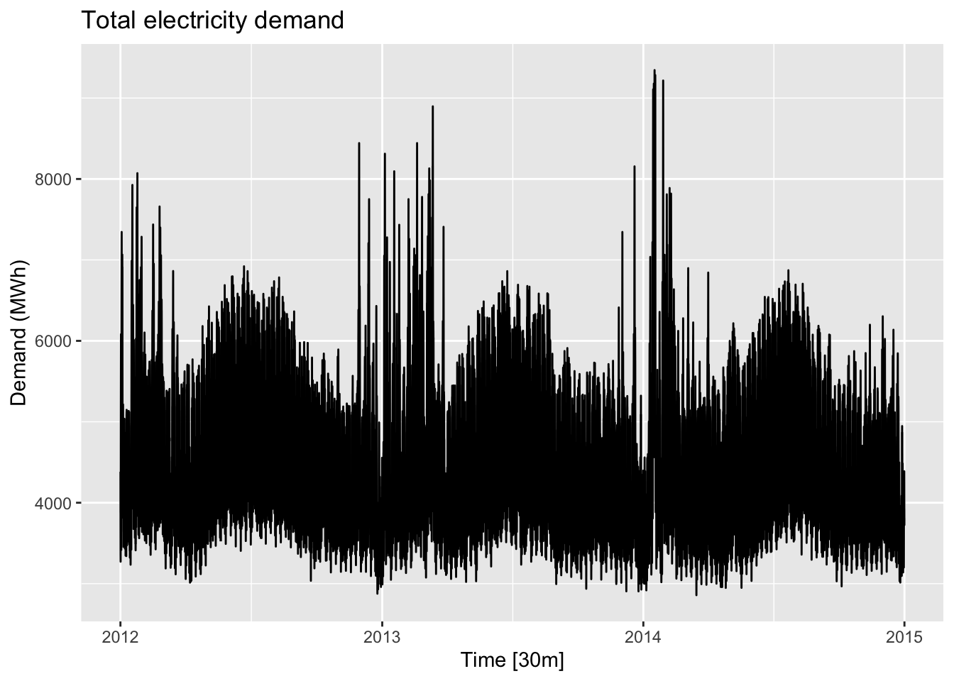

peak_stock <- gafa_stock |>
  group_by(Symbol) |>
  filter(Close == max(Close)) |>
  select(Close) |>
  ungroup()

## Adding missing grouping variables: `Symbol`

peak_stock

## # A tsibble: 4 x 3 [!]
## # Key:       Symbol [4]
##   Symbol Close Date      
##   <chr>  <dbl> <date>    
## 1 AAPL    232. 2018-10-03
## 2 AMZN   2040. 2018-09-04
## 3 FB      218. 2018-07-25
## 4 GOOG   1268. 2018-07-26

gafa_stock |>
  autoplot(Close) + 
  geom_vline(data=peak_stock, mapping=aes(xintercept=Date), color = 'red') +
  geom_point(data=peak_stock, mapping=aes(x=Date, y=Close), color = 'red') +
  facet_grid(vars(Symbol), scale = 'free_y') +
  labs(y = '$USD', title = 'Historical stock prices from 2014-2018',
       subtitle = 'Google, Amazon, Facebook and Apple')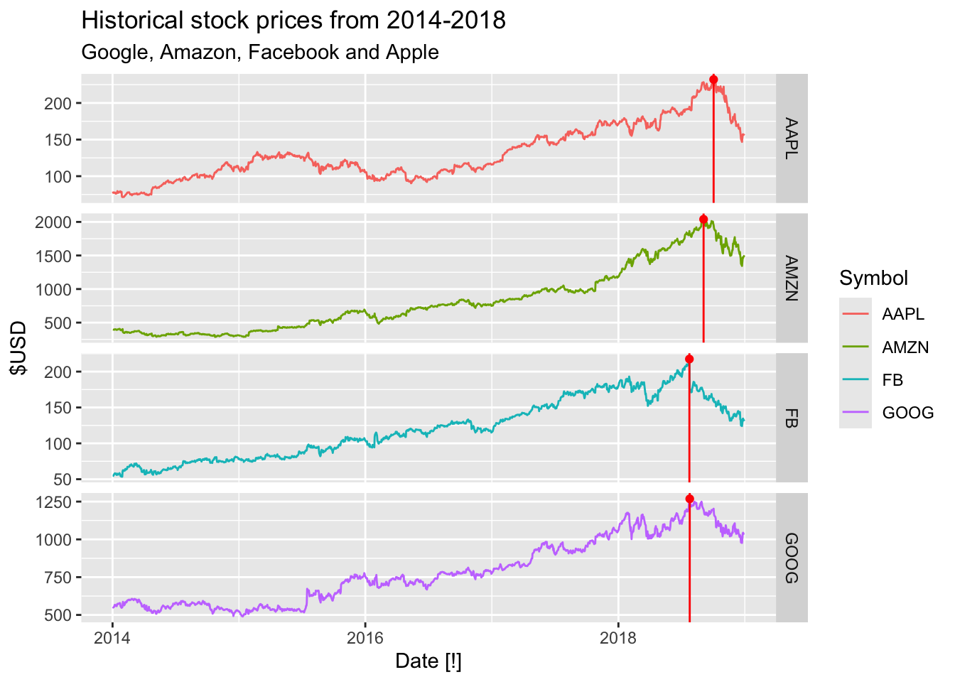

# a.
tute <- import('https://bit.ly/fpptute1')
tute

##        Quarter  Sales AdBudget   GDP
## 1   1981-03-01 1020.2    659.2 251.8
## 2   1981-06-01  889.2    589.0 290.9
## 3   1981-09-01  795.0    512.5 290.8
## 4   1981-12-01 1003.9    614.1 292.4
## 5   1982-03-01 1057.7    647.2 279.1
## 6   1982-06-01  944.4    602.0 254.0
## 7   1982-09-01  778.5    530.7 295.6
## 8   1982-12-01  932.5    608.4 271.7
## 9   1983-03-01  996.5    637.9 259.6
## 10  1983-06-01  907.7    582.4 280.5
## 11  1983-09-01  735.1    506.8 287.2
## 12  1983-12-01  958.1    606.7 278.0
## 13  1984-03-01 1034.1    658.7 256.8
## 14  1984-06-01  992.8    614.9 271.0
## 15  1984-09-01  791.7    489.9 300.9
## 16  1984-12-01  914.2    586.5 289.8
## 17  1985-03-01 1106.5    663.0 266.8
## 18  1985-06-01  985.1    591.7 273.7
## 19  1985-09-01  823.9    502.2 301.3
## 20  1985-12-01 1025.1    616.4 285.6
## 21  1986-03-01 1064.7    647.1 270.6
## 22  1986-06-01  981.9    615.5 274.6
## 23  1986-09-01  828.3    514.8 299.7
## 24  1986-12-01  940.7    609.1 275.9
## 25  1987-03-01  991.1    641.3 279.3
## 26  1987-06-01 1021.2    620.2 290.8
## 27  1987-09-01  796.7    511.2 295.6
## 28  1987-12-01  986.6    621.3 271.9
## 29  1988-03-01 1054.2    645.3 267.4
## 30  1988-06-01 1018.7    616.0 281.0
## 31  1988-09-01  815.6    503.2 309.0
## 32  1988-12-01 1010.6    617.5 266.7
## 33  1989-03-01 1071.5    642.8 283.5
## 34  1989-06-01  954.0    585.6 282.3
## 35  1989-09-01  822.9    520.6 289.2
## 36  1989-12-01  867.5    608.6 270.7
## 37  1990-03-01 1002.3    645.7 266.5
## 38  1990-06-01  972.0    597.4 287.9
## 39  1990-09-01  782.9    499.8 287.6
## 40  1990-12-01  972.8    601.8 283.4
## 41  1991-03-01 1108.0    650.8 266.4
## 42  1991-06-01  943.7    588.3 292.3
## 43  1991-09-01  806.1    491.6 330.6
## 44  1991-12-01  954.2    603.3 286.2
## 45  1992-03-01 1115.5    663.2 259.2
## 46  1992-06-01  927.1    614.0 263.7
## 47  1992-09-01  800.7    506.3 288.2
## 48  1992-12-01  955.7    606.2 274.1
## 49  1993-03-01 1049.8    639.5 287.1
## 50  1993-06-01  886.0    585.9 285.5
## 51  1993-09-01  786.4    492.2 303.7
## 52  1993-12-01  991.3    610.4 275.6
## 53  1994-03-01 1113.9    660.8 249.3
## 54  1994-06-01  924.5    612.2 272.9
## 55  1994-09-01  771.4    509.2 289.8
## 56  1994-12-01  949.8    612.1 269.2
## 57  1995-03-01  990.5    653.2 261.3
## 58  1995-06-01 1071.4    605.3 292.9
## 59  1995-09-01  854.1    506.6 304.6
## 60  1995-12-01  929.8    597.4 276.3
## 61  1996-03-01  959.6    635.2 268.2
## 62  1996-06-01  991.1    611.6 293.5
## 63  1996-09-01  832.9    503.8 311.1
## 64  1996-12-01 1006.1    609.9 273.7
## 65  1997-03-01 1040.7    645.2 267.5
## 66  1997-06-01 1026.3    609.8 271.9
## 67  1997-09-01  785.9    512.1 308.8
## 68  1997-12-01  997.6    603.7 282.9
## 69  1998-03-01 1055.0    639.4 268.4
## 70  1998-06-01  925.6    601.6 271.4
## 71  1998-09-01  805.6    497.0 292.1
## 72  1998-12-01  934.1    602.8 287.6
## 73  1999-03-01 1081.7    647.3 258.0
## 74  1999-06-01 1062.3    612.5 282.9
## 75  1999-09-01  798.8    492.2 295.0
## 76  1999-12-01 1014.3    610.8 271.2
## 77  2000-03-01 1049.5    646.5 275.4
## 78  2000-06-01  961.7    603.3 284.0
## 79  2000-09-01  793.4    503.8 300.9
## 80  2000-12-01  872.3    598.3 277.4
## 81  2001-03-01 1014.2    649.4 273.8
## 82  2001-06-01  952.6    620.2 288.4
## 83  2001-09-01  792.4    497.9 283.4
## 84  2001-12-01  922.3    609.2 273.4
## 85  2002-03-01 1055.9    665.9 271.5
## 86  2002-06-01  906.2    600.4 283.6
## 87  2002-09-01  811.2    502.3 290.6
## 88  2002-12-01 1005.8    605.6 289.1
## 89  2003-03-01 1013.8    647.6 282.2
## 90  2003-06-01  905.6    583.5 285.6
## 91  2003-09-01  957.3    502.5 304.0
## 92  2003-12-01 1059.5    625.9 271.5
## 93  2004-03-01 1090.6    648.7 263.9
## 94  2004-06-01  998.9    610.7 288.3
## 95  2004-09-01  866.6    519.1 290.2
## 96  2004-12-01 1018.7    634.9 284.0
## 97  2005-03-01 1112.5    663.1 270.9
## 98  2005-06-01  997.4    583.3 294.7
## 99  2005-09-01  826.8    508.6 292.2
## 100 2005-12-01  992.6    634.2 255.1

str(tute)

## 'data.frame':    100 obs. of  4 variables:
##  $ Quarter : IDate, format: "1981-03-01" "1981-06-01" "1981-09-01" "1981-12-01" ...
##  $ Sales   : num  1020 889 795 1004 1058 ...
##  $ AdBudget: num  659 589 512 614 647 ...
##  $ GDP     : num  252 291 291 292 279 ...

# b.
tute |>
   mutate(Quarter = yearquarter(Quarter)) |>
  as_tsibble(index = Quarter)

## # A tsibble: 100 x 4 [1Q]
##    Quarter Sales AdBudget   GDP
##      <qtr> <dbl>    <dbl> <dbl>
##  1 1981 Q1 1020.     659.  252.
##  2 1981 Q2  889.     589   291.
##  3 1981 Q3  795      512.  291.
##  4 1981 Q4 1004.     614.  292.
##  5 1982 Q1 1058.     647.  279.
##  6 1982 Q2  944.     602   254 
##  7 1982 Q3  778.     531.  296.
##  8 1982 Q4  932.     608.  272.
##  9 1983 Q1  996.     638.  260.
## 10 1983 Q2  908.     582.  280.
## # ℹ 90 more rows

# c.

tute |>
   mutate(Quarter = yearquarter(Quarter)) |>
   as_tsibble(index = Quarter) |>
   pivot_longer(-Quarter) |>
   ggplot(aes(x = Quarter, y = value, color = name)) +
      geom_line()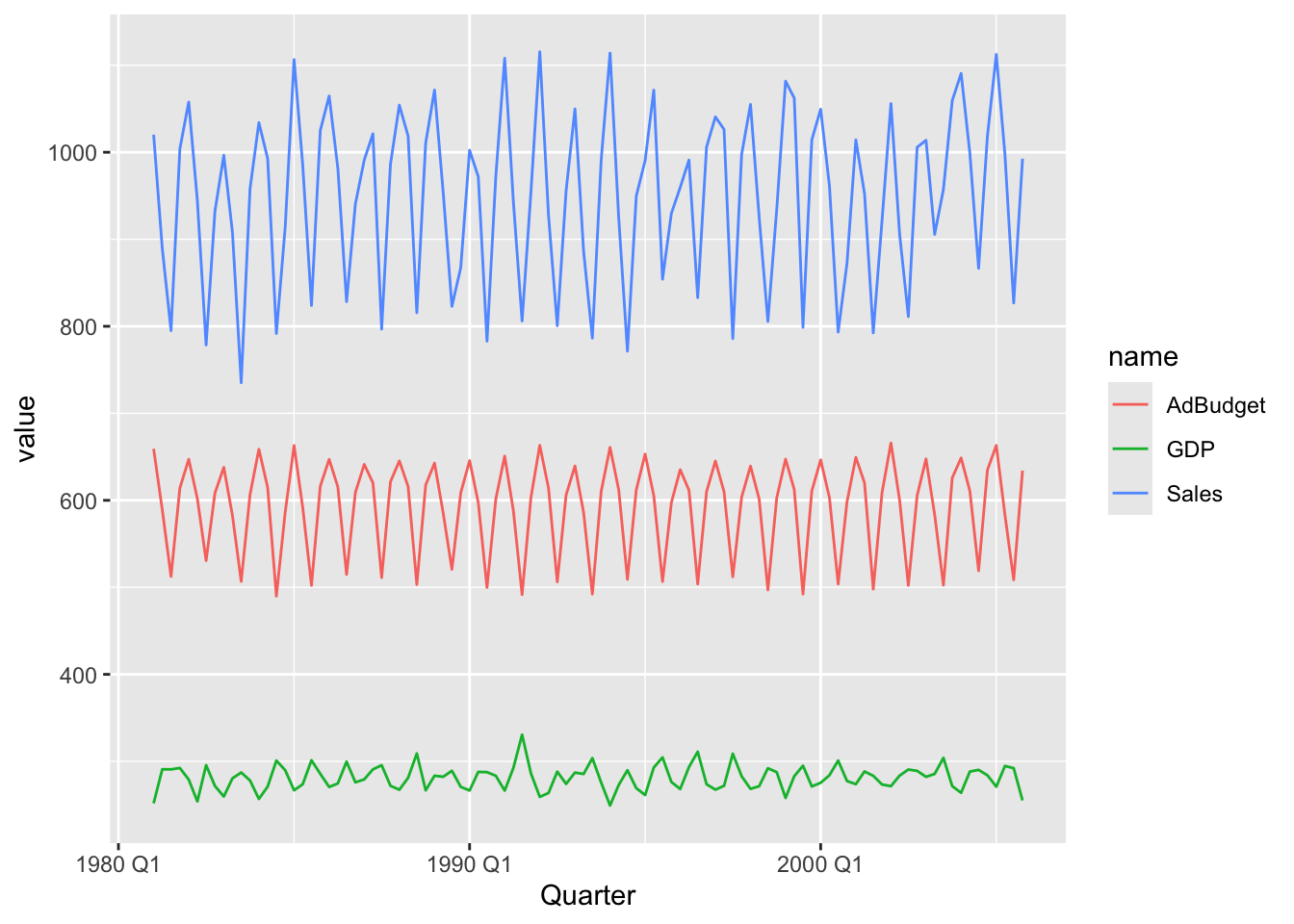

tute |>
   mutate(Quarter = yearquarter(Quarter)) |>
   as_tsibble(index = Quarter) |>
   pivot_longer(-Quarter) |>
   autoplot()

## Plot variable not specified, automatically selected `.vars = value`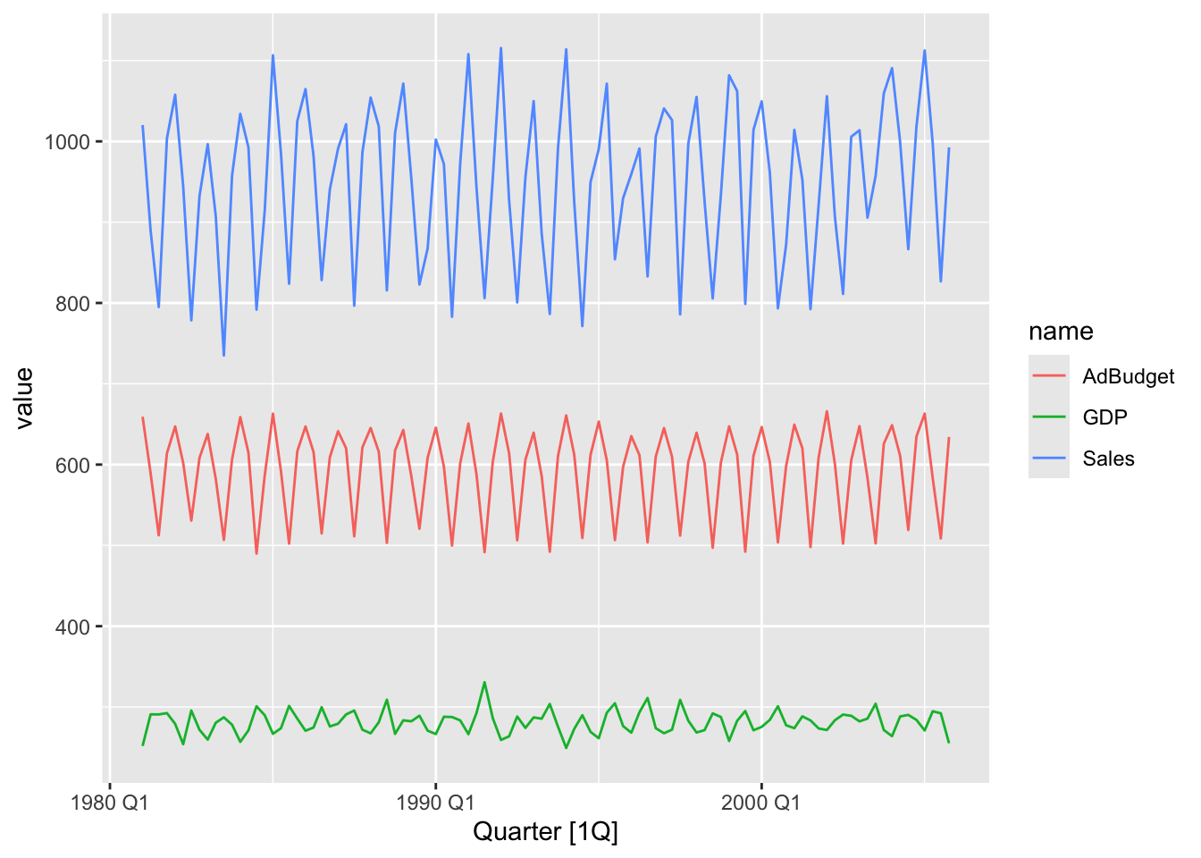

# split time series into different plots
tute |>
   mutate(Quarter = yearquarter(Quarter)) |>
   as_tsibble(index = Quarter) |>
   pivot_longer(-Quarter) |>
   ggplot(aes(x = Quarter, y = value, color = name)) +
      geom_line() +
   facet_grid(name ~ ., scales = "free_y")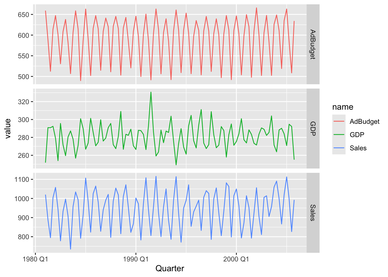

# a.

# load library
library(USgas)

?us_total

# b.
us_total |>
  as_tsibble(index = year, key = c(state))

## # A tsibble: 1,266 x 3 [1Y]
## # Key:       state [53]
##     year state        y
##    <int> <chr>    <int>
##  1  1997 Alabama 324158
##  2  1998 Alabama 329134
##  3  1999 Alabama 337270
##  4  2000 Alabama 353614
##  5  2001 Alabama 332693
##  6  2002 Alabama 379343
##  7  2003 Alabama 350345
##  8  2004 Alabama 382367
##  9  2005 Alabama 353156
## 10  2006 Alabama 391093
## # ℹ 1,256 more rows

# c.
us_total |>
  as_tsibble(index = year, key = c(state)) |>
  filter(state %in% c('Maine', 'Vermont', 'New Hampshire', 
                      'Massachusetts', 'Connecticut', 'Rhode Island')) |>
  autoplot() +
  labs(y = 'Volume (Million Cubic Feet)',
       title = 'Annual natural gas consumption',
       subtitle = 'New England area')

## Plot variable not specified, automatically selected `.vars = y`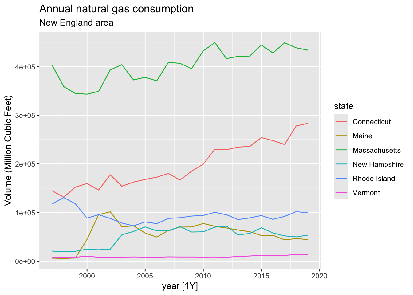

# a.
tourism.5 <- import('https://bit.ly/fpptourism')

# b.

# tourism form tsibble package
tourism

## # A tsibble: 24,320 x 5 [1Q]
## # Key:       Region, State, Purpose [304]
##    Quarter Region   State Purpose  Trips
##      <qtr> <chr>    <chr> <chr>    <dbl>
##  1 1998 Q1 Adelaide SA    Business  135.
##  2 1998 Q2 Adelaide SA    Business  110.
##  3 1998 Q3 Adelaide SA    Business  166.
##  4 1998 Q4 Adelaide SA    Business  127.
##  5 1999 Q1 Adelaide SA    Business  137.
##  6 1999 Q2 Adelaide SA    Business  200.
##  7 1999 Q3 Adelaide SA    Business  169.
##  8 1999 Q4 Adelaide SA    Business  134.
##  9 2000 Q1 Adelaide SA    Business  154.
## 10 2000 Q2 Adelaide SA    Business  169.
## # ℹ 24,310 more rows

# index = Quarter, keys = [Region, State, Purpose]

ts_tourims <- tourism.5 |>
  mutate(Quarter = yearquarter(Quarter)) |>
  as_tsibble(index = Quarter,
             key = c('Region', 'State', 'Purpose'))

ts_tourims

## # A tsibble: 24,320 x 5 [1Q]
## # Key:       Region, State, Purpose [304]
##    Quarter Region   State           Purpose  Trips
##      <qtr> <chr>    <chr>           <chr>    <dbl>
##  1 1998 Q1 Adelaide South Australia Business  135.
##  2 1998 Q2 Adelaide South Australia Business  110.
##  3 1998 Q3 Adelaide South Australia Business  166.
##  4 1998 Q4 Adelaide South Australia Business  127.
##  5 1999 Q1 Adelaide South Australia Business  137.
##  6 1999 Q2 Adelaide South Australia Business  200.
##  7 1999 Q3 Adelaide South Australia Business  169.
##  8 1999 Q4 Adelaide South Australia Business  134.
##  9 2000 Q1 Adelaide South Australia Business  154.
## 10 2000 Q2 Adelaide South Australia Business  169.
## # ℹ 24,310 more rows

# c.
ts_tourims |> distinct(Region)

## # A tibble: 76 × 1
##    Region                    
##    <chr>                     
##  1 Adelaide                  
##  2 Adelaide Hills            
##  3 Alice Springs             
##  4 Australia's Coral Coast   
##  5 Australia's Golden Outback
##  6 Australia's North West    
##  7 Australia's South West    
##  8 Ballarat                  
##  9 Barkly                    
## 10 Barossa                   
## # ℹ 66 more rows

ts_tourims |> distinct(Purpose)

## # A tibble: 4 × 1
##   Purpose 
##   <chr>   
## 1 Business
## 2 Holiday 
## 3 Other   
## 4 Visiting

ts_tourims |>
  group_by(Region, Purpose) |>
  summarise(Trips = mean(Trips)) |>
  arrange(desc(Trips)) |>
  slice(1)

## Warning: Current temporal ordering may yield unexpected results.
## ℹ Suggest to sort by `Region`, `Purpose`, `Quarter` first.

## # A tsibble: 76 x 4 [1Q]
## # Key:       Region, Purpose [76]
## # Groups:    Region [76]
##    Region                     Purpose  Quarter Trips
##    <chr>                      <chr>      <qtr> <dbl>
##  1 Adelaide                   Visiting 2017 Q1 270. 
##  2 Adelaide Hills             Visiting 2002 Q4  81.1
##  3 Alice Springs              Holiday  1998 Q3  76.5
##  4 Australia's Coral Coast    Holiday  2014 Q3 198. 
##  5 Australia's Golden Outback Business 2017 Q3 174. 
##  6 Australia's North West     Business 2016 Q3 297. 
##  7 Australia's South West     Holiday  2016 Q1 612. 
##  8 Ballarat                   Visiting 2004 Q1 103. 
##  9 Barkly                     Holiday  1998 Q3  37.9
## 10 Barossa                    Holiday  2006 Q1  51.0
## # ℹ 66 more rows

#d.
ts_tourims |>
  group_by(State) |>
  summarise(total_trips = sum(Trips)) |>
  as_tsibble(index = Quarter, key = c(State))

## # A tsibble: 640 x 3 [1Q]
## # Key:       State [8]
##    State Quarter total_trips
##    <chr>   <qtr>       <dbl>
##  1 ACT   1998 Q1        551.
##  2 ACT   1998 Q2        416.
##  3 ACT   1998 Q3        436.
##  4 ACT   1998 Q4        450.
##  5 ACT   1999 Q1        379.
##  6 ACT   1999 Q2        558.
##  7 ACT   1999 Q3        449.
##  8 ACT   1999 Q4        595.
##  9 ACT   2000 Q1        600.
## 10 ACT   2000 Q2        557.
## # ℹ 630 more rows

?aus_arrivals
aus_arrivals

## # A tsibble: 508 x 3 [1Q]
## # Key:       Origin [4]
##    Quarter Origin Arrivals
##      <qtr> <chr>     <int>
##  1 1981 Q1 Japan     14763
##  2 1981 Q2 Japan      9321
##  3 1981 Q3 Japan     10166
##  4 1981 Q4 Japan     19509
##  5 1982 Q1 Japan     17117
##  6 1982 Q2 Japan     10617
##  7 1982 Q3 Japan     11737
##  8 1982 Q4 Japan     20961
##  9 1983 Q1 Japan     20671
## 10 1983 Q2 Japan     12235
## # ℹ 498 more rows

# autoplot()
aus_arrivals |>
  autoplot(Arrivals) +
  facet_grid(vars(Origin), scales = 'free_y') +
  labs(title = 'Quarterly international arrivals to Australia')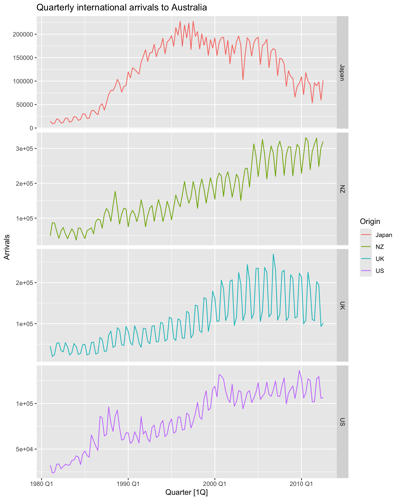

# gg_season()
aus_arrivals |>
  gg_season(Arrivals, labels = 'both') +
  facet_grid(vars(Origin), scales = 'free_y') +
  labs(title = 'Seasonal international arrivals to Australia')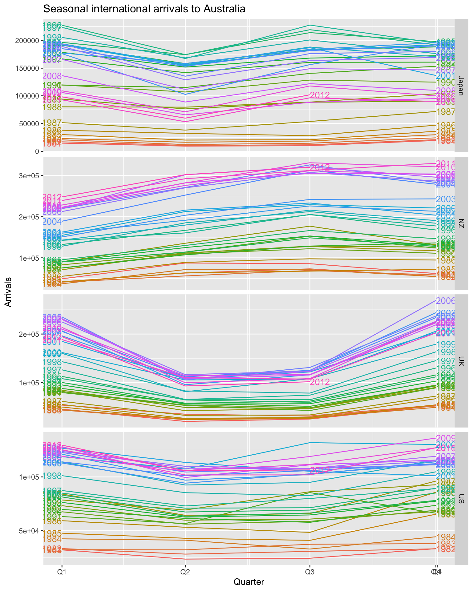

# gg_subseries()
aus_arrivals |>
  gg_subseries(Arrivals) +
  labs(title = 'Quarterly international arrivals to Australia')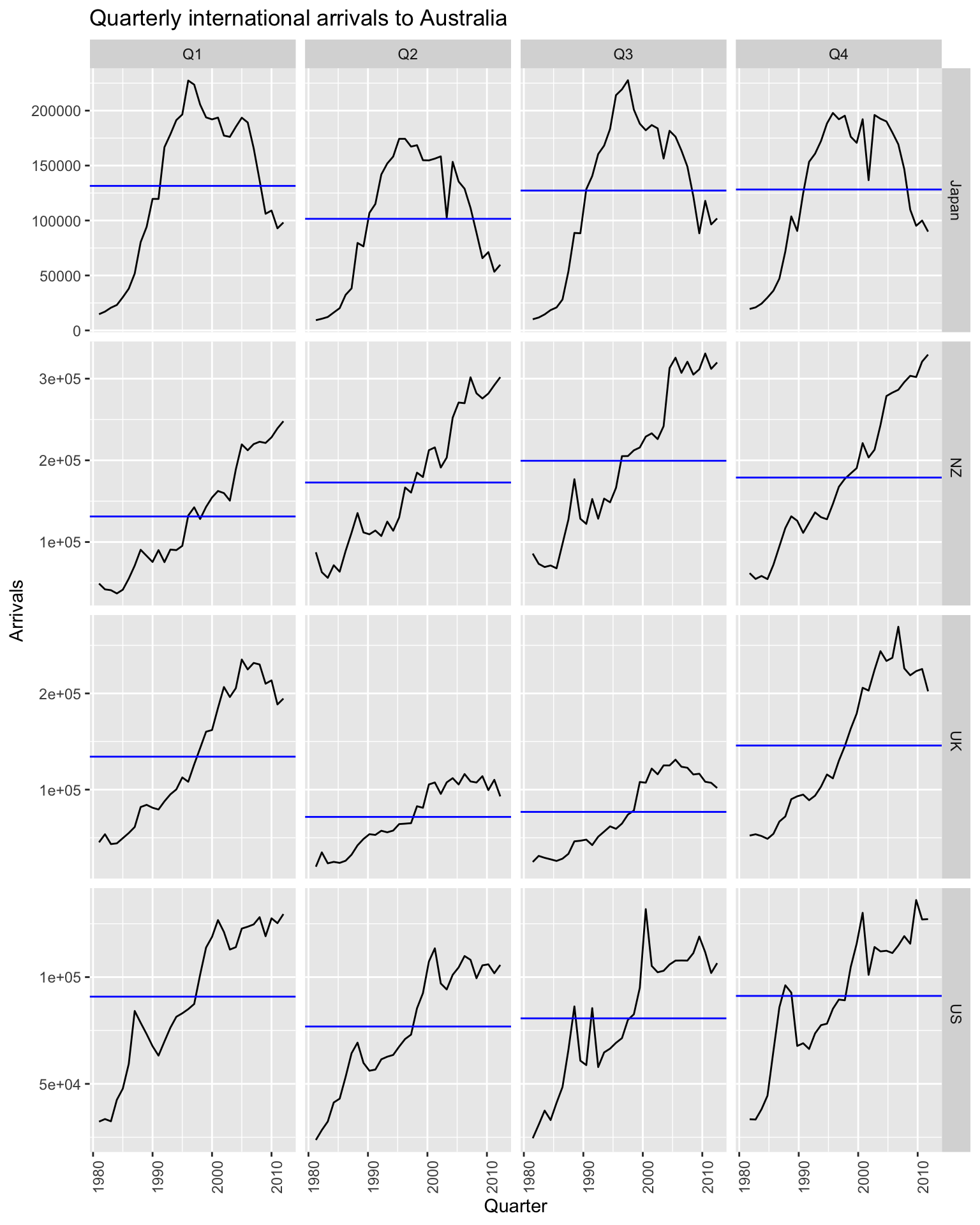

?aus_retail
aus_retail

## # A tsibble: 64,532 x 5 [1M]
## # Key:       State, Industry [152]
##    State                        Industry                                 `Series ID`    Month Turnover
##    <chr>                        <chr>                                    <chr>          <mth>    <dbl>
##  1 Australian Capital Territory Cafes, restaurants and catering services A3349849A   1982 Apr      4.4
##  2 Australian Capital Territory Cafes, restaurants and catering services A3349849A   1982 May      3.4
##  3 Australian Capital Territory Cafes, restaurants and catering services A3349849A   1982 Jun      3.6
##  4 Australian Capital Territory Cafes, restaurants and catering services A3349849A   1982 Jul      4  
##  5 Australian Capital Territory Cafes, restaurants and catering services A3349849A   1982 Aug      3.6
##  6 Australian Capital Territory Cafes, restaurants and catering services A3349849A   1982 Sep      4.2
##  7 Australian Capital Territory Cafes, restaurants and catering services A3349849A   1982 Oct      4.8
##  8 Australian Capital Territory Cafes, restaurants and catering services A3349849A   1982 Nov      5.4
##  9 Australian Capital Territory Cafes, restaurants and catering services A3349849A   1982 Dec      6.9
## 10 Australian Capital Territory Cafes, restaurants and catering services A3349849A   1983 Jan      3.8
## # ℹ 64,522 more rows

myseries <- aus_retail |>
  filter(`Series ID` == sample(aus_retail$`Series ID`,1))

myseries

## # A tsibble: 441 x 5 [1M]
## # Key:       State, Industry [1]
##    State    Industry                           `Series ID`    Month Turnover
##    <chr>    <chr>                              <chr>          <mth>    <dbl>
##  1 Victoria Other recreational goods retailing A3349415T   1982 Apr     15.6
##  2 Victoria Other recreational goods retailing A3349415T   1982 May     15.8
##  3 Victoria Other recreational goods retailing A3349415T   1982 Jun     15.2
##  4 Victoria Other recreational goods retailing A3349415T   1982 Jul     15.2
##  5 Victoria Other recreational goods retailing A3349415T   1982 Aug     14.5
##  6 Victoria Other recreational goods retailing A3349415T   1982 Sep     15.1
##  7 Victoria Other recreational goods retailing A3349415T   1982 Oct     16.3
##  8 Victoria Other recreational goods retailing A3349415T   1982 Nov     17.5
##  9 Victoria Other recreational goods retailing A3349415T   1982 Dec     21.5
## 10 Victoria Other recreational goods retailing A3349415T   1983 Jan     15.6
## # ℹ 431 more rows

myseries |>
  autoplot()

## Plot variable not specified, automatically selected `.vars = Turnover`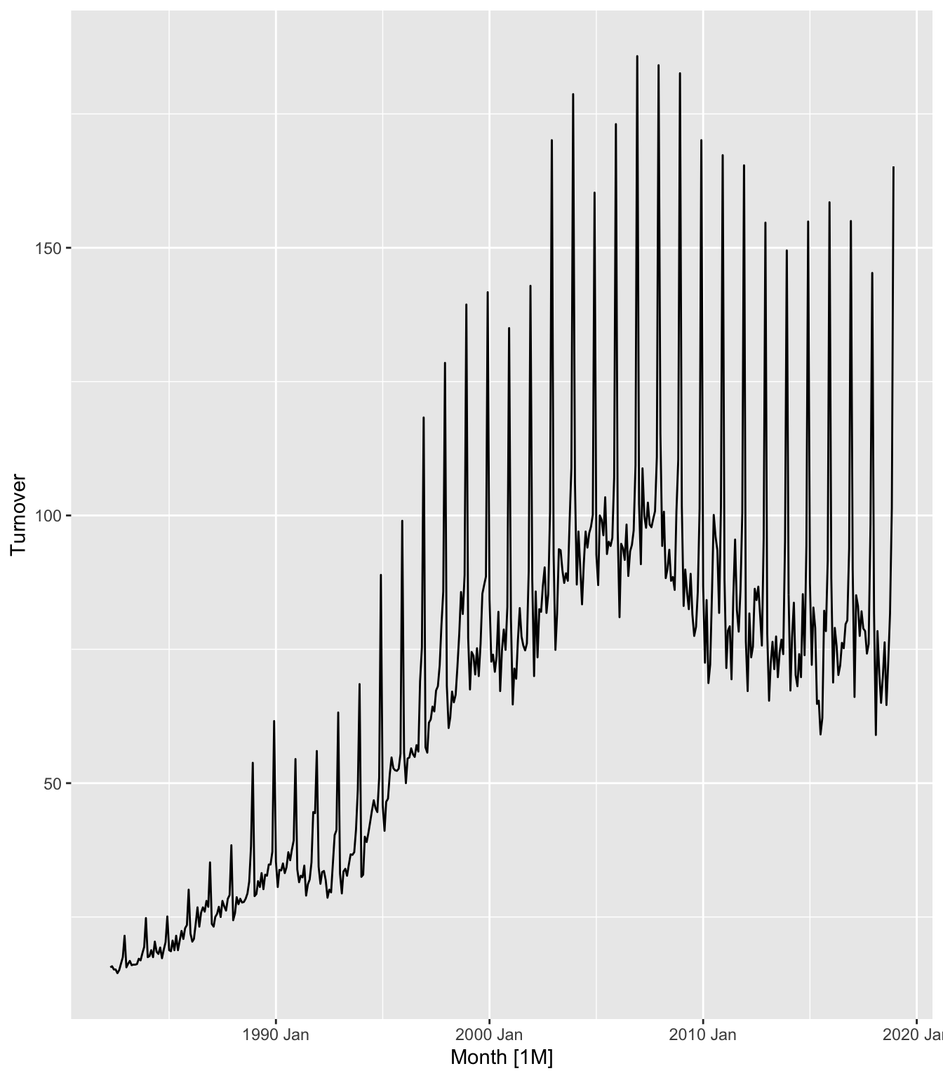

myseries |>
  gg_season(labels = 'both')

## Plot variable not specified, automatically selected `y = Turnover`

myseries |>
  gg_subseries()

## Plot variable not specified, automatically selected `y = Turnover`

myseries |>
  gg_lag(geom = 'point')

## Plot variable not specified, automatically selected `y = Turnover`

myseries |>
  gg_tsdisplay()

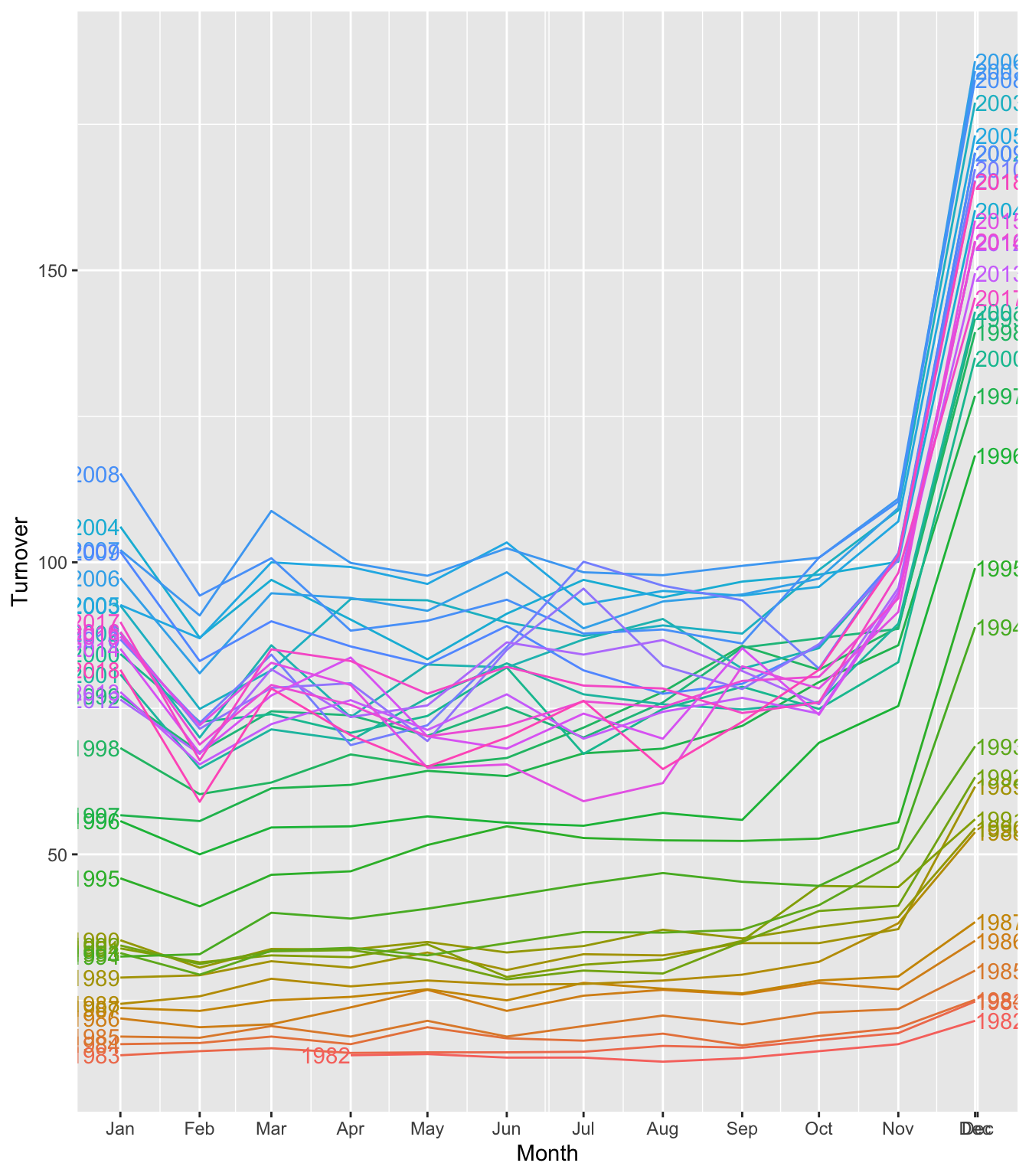
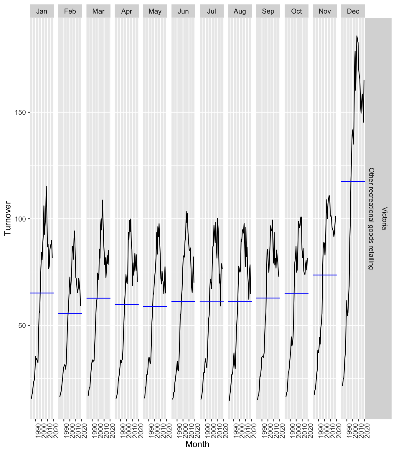
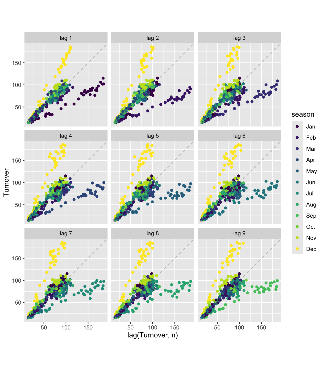
## Plot variable not specified, automatically selected `y = Turnover`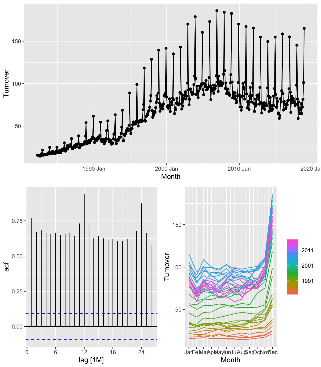

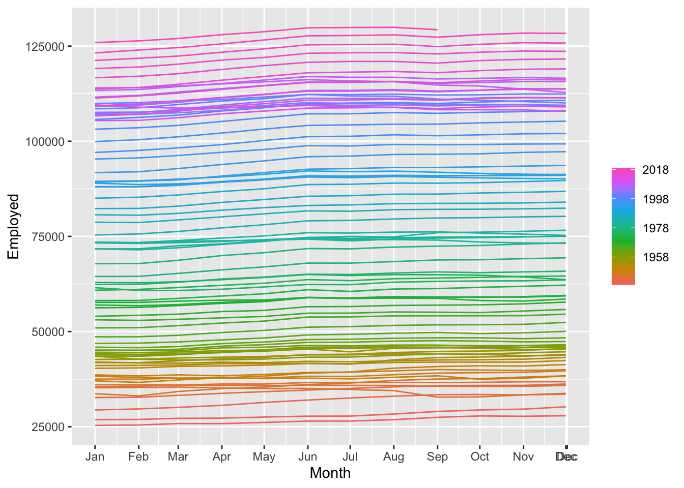
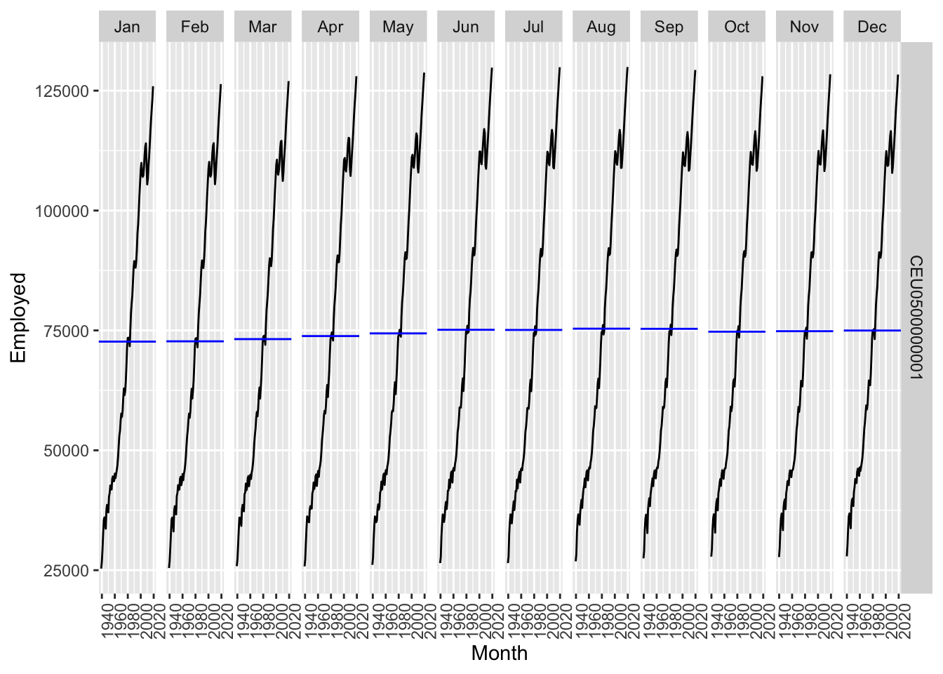
# “Total Private” Employed from us_employment
total_private <- us_employment |>
  filter(Title == 'Total Private')

total_private |> autoplot(Employed)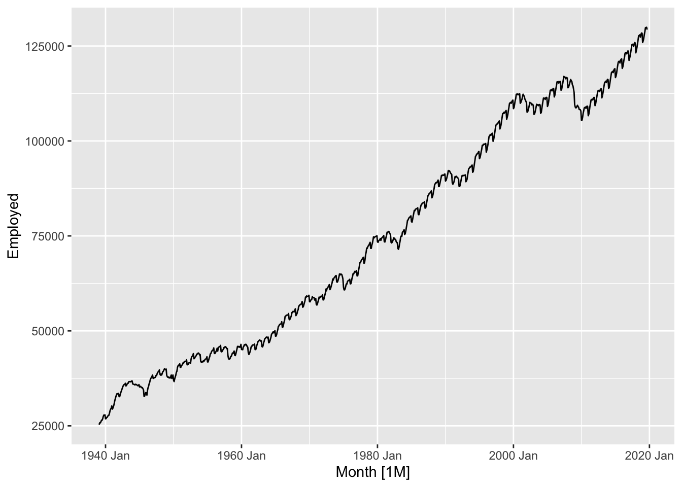

total_private |> gg_season(Employed)

total_private |> gg_subseries(Employed)

total_private |> gg_lag(Employed)

total_private |> ACF(Employed) |> autoplot()

# Bricks from aus_production
aus_production |> autoplot(Bricks)

## Warning: Removed 20 rows containing missing values or values outside the scale range (`geom_line()`).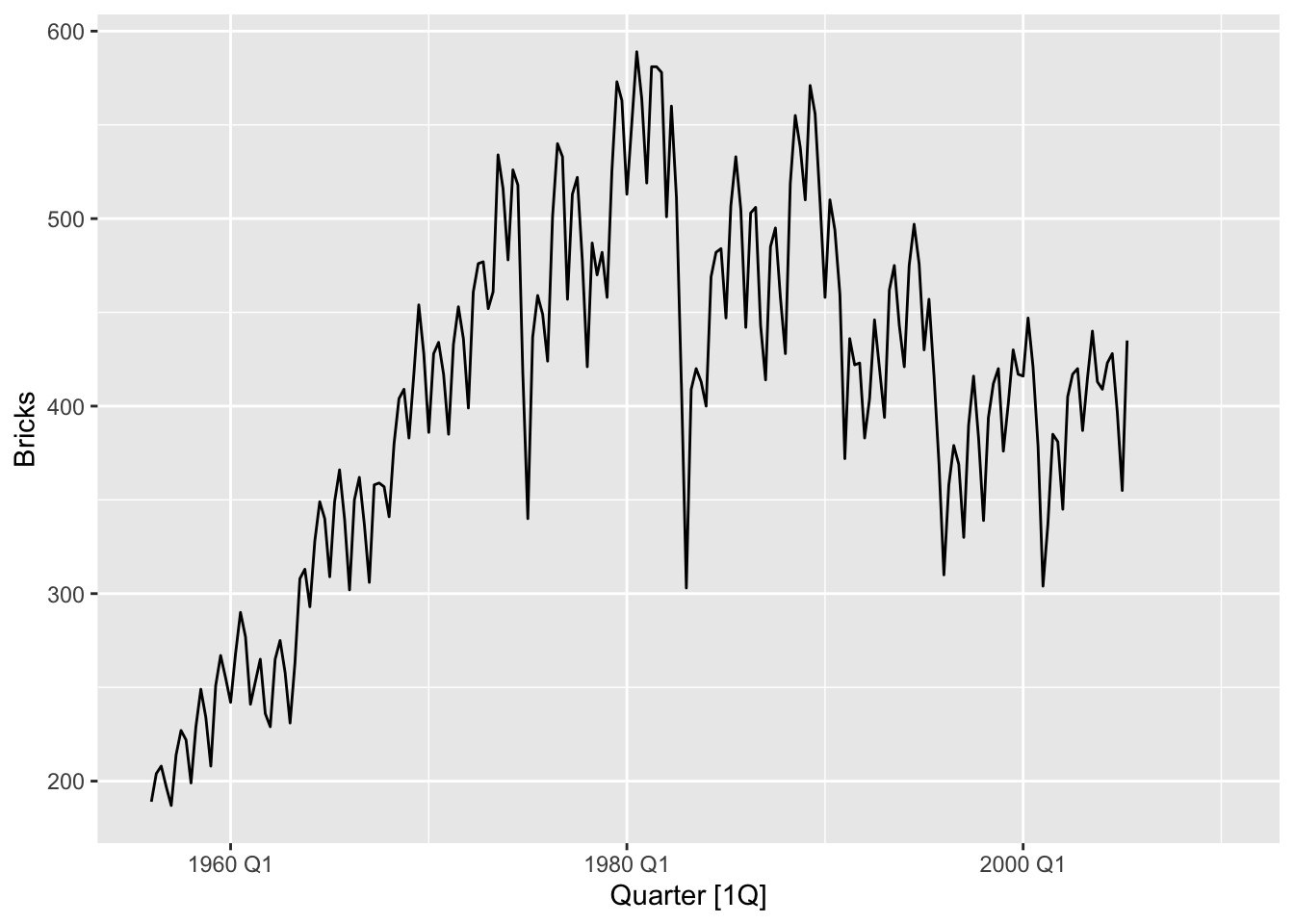

aus_production |> gg_season(Bricks, labels = 'both')

## Warning: Removed 20 rows containing missing values or values outside the scale range (`geom_line()`).

## Warning: Removed 5 rows containing missing values or values outside the scale range (`geom_text()`).

## Warning: Removed 6 rows containing missing values or values outside the scale range (`geom_text()`).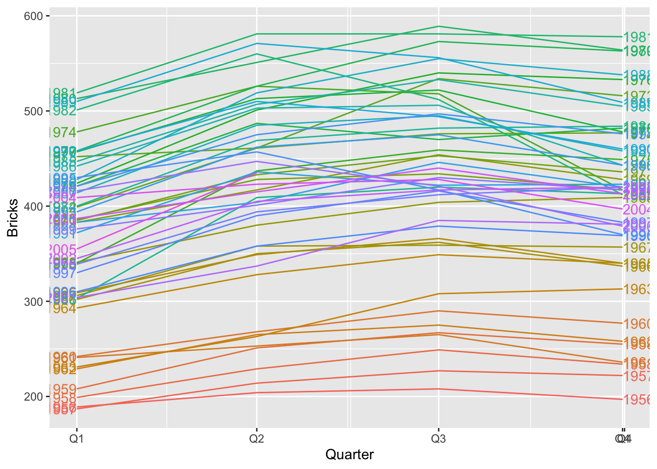

aus_production |> gg_subseries(Bricks)

## Warning: Removed 5 rows containing missing values or values outside the scale range (`geom_line()`).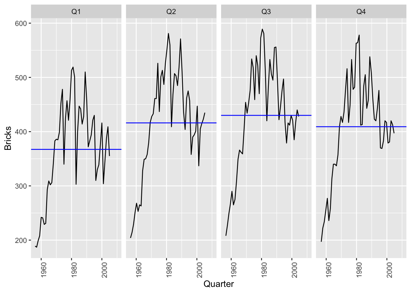

aus_production |> gg_lag(Bricks)

## Warning: Removed 20 rows containing missing values (gg_lag).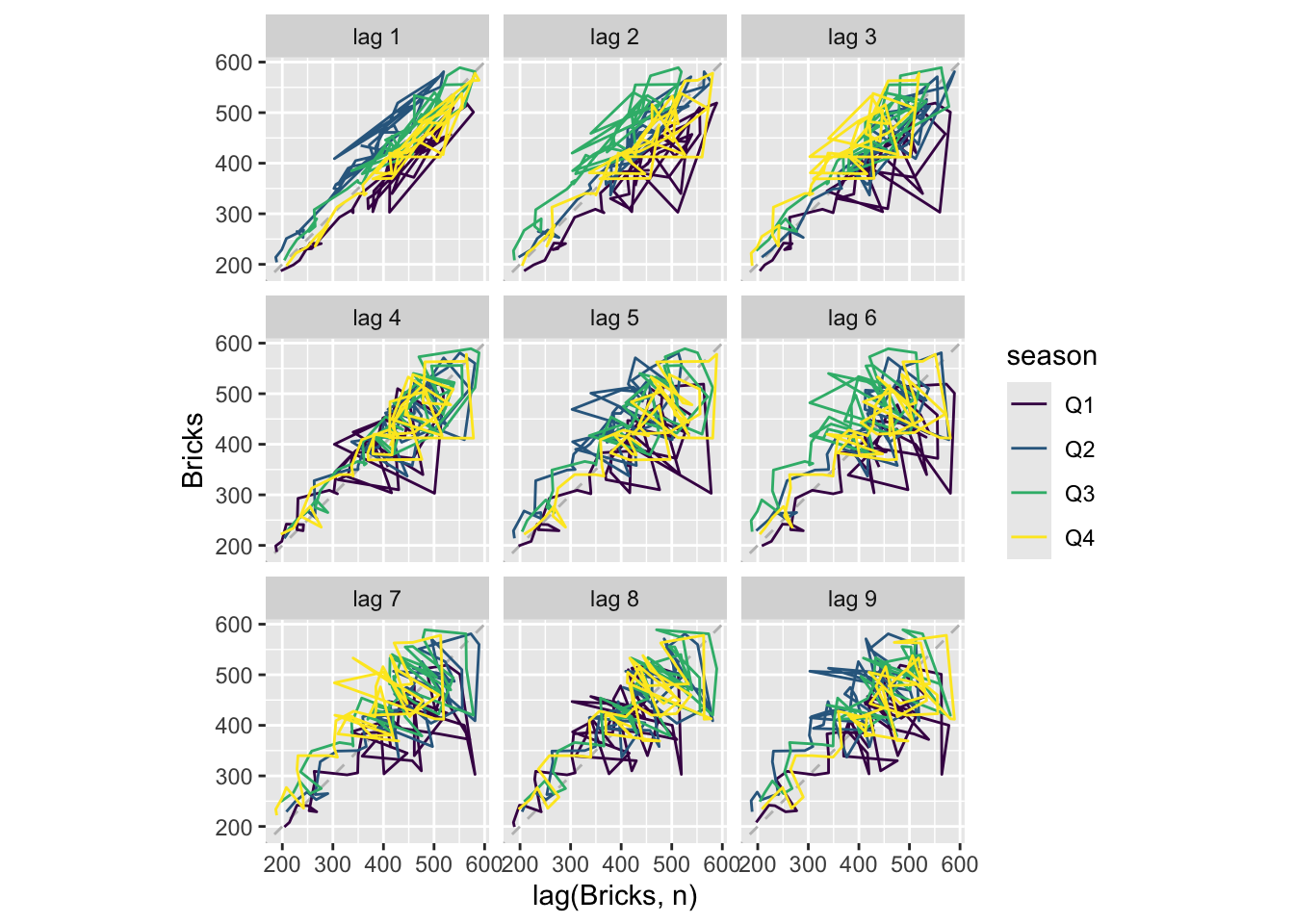

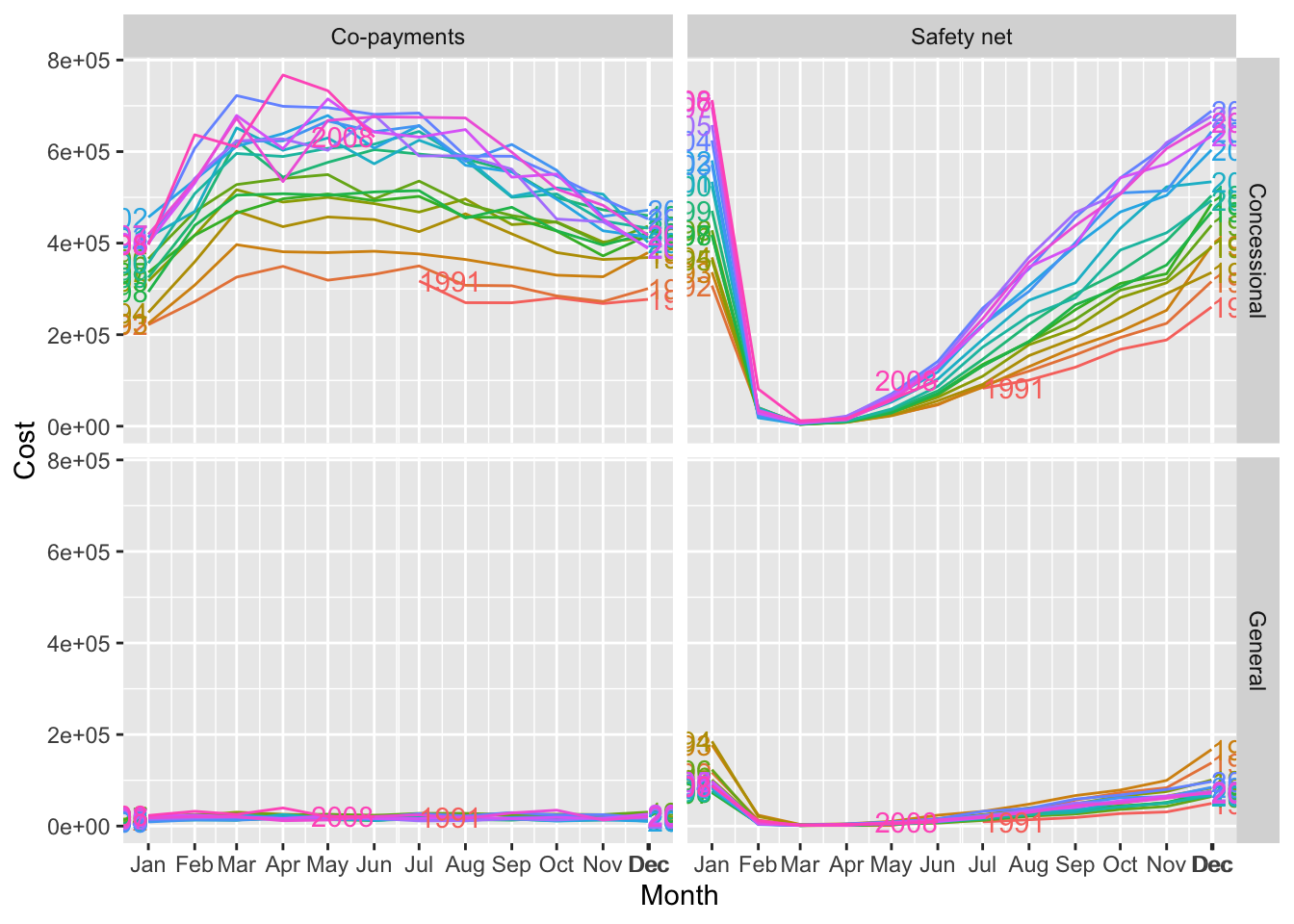
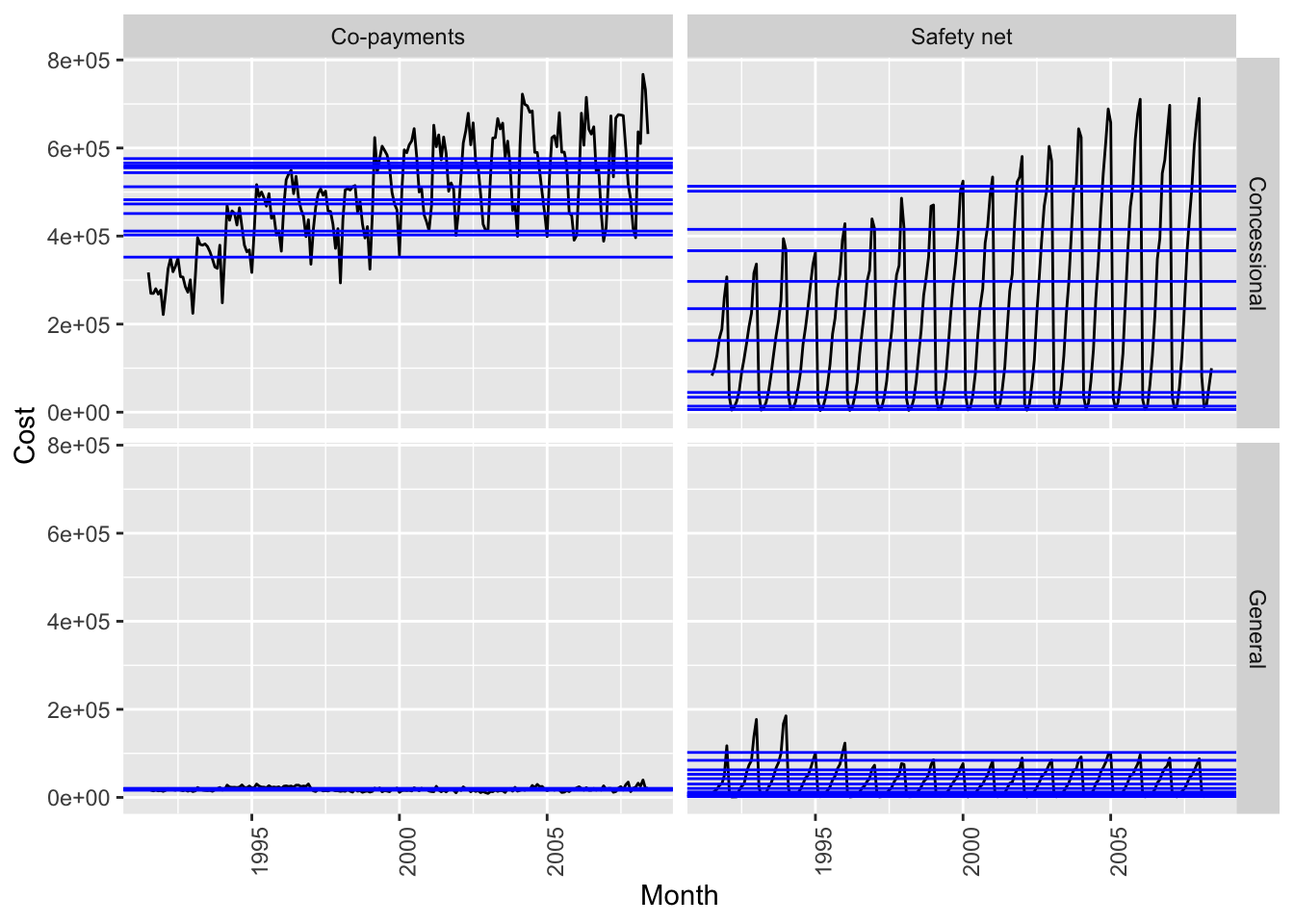
aus_production |> ACF(Bricks) |> autoplot()

# Hare from pelt
pelt |> autoplot(Hare)

#pelt |> gg_season(Hare, labels = "both")
pelt |> gg_subseries(Hare)

pelt |> gg_lag(Hare)

pelt |> ACF(Hare) |> autoplot()

# “H02” Cost from PBS

h02 <- PBS |>
  filter(ATC2 == 'H02') |>
  select(Cost) |>
  as_tsibble(index = Month, key = c("Concession", "Type", "ATC1", "ATC2"))
  
h02 |> autoplot(Cost) +
  facet_grid(Concession ~ Type) +
  theme(legend.position="none")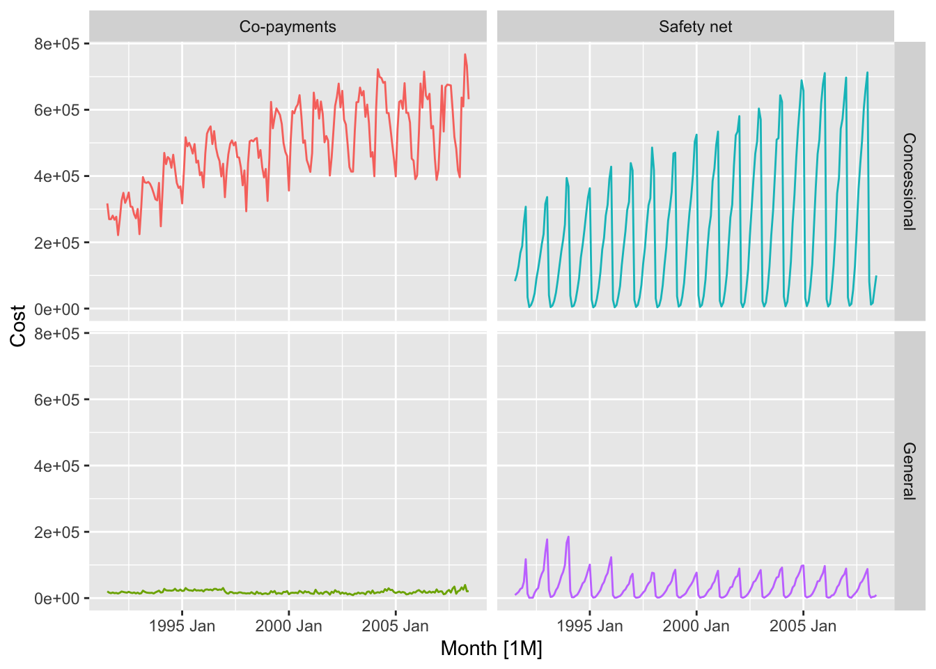

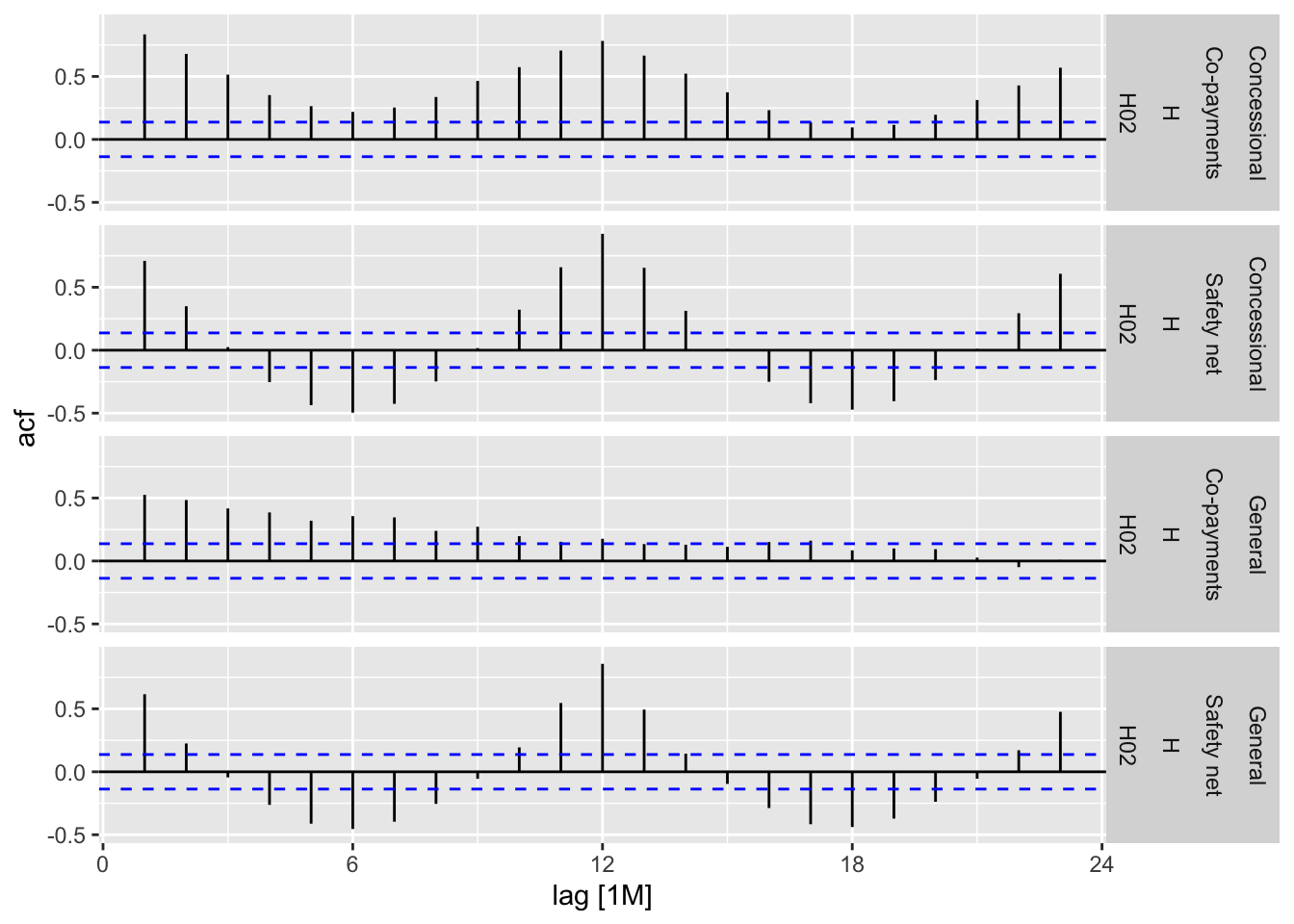
h02 |> gg_season(Cost, labels = 'both') +
  facet_grid(Concession ~ Type)

h02 |> gg_subseries(Cost) +
  facet_grid(Concession ~ Type)

# h02 |> gg_lag(Cost) +
#   facet_grid(Concession ~ Type)

h02 |> ACF(Cost) |> autoplot()

# Barrels from us_gasoline
us_gasoline |> autoplot(Barrels)

us_gasoline |> gg_season(Barrels, labels = 'both')

us_gasoline |> gg_subseries(Barrels)

us_gasoline |> gg_lag(Barrels)

us_gasoline |> ACF(Barrels) |> autoplot()

Source: #9 in 2.10 Exercises section

# 1 - B
# 2 - A
# 3 - D
# 4 - C

library(fma)
# 1
cowtemp |> autoplot()

cowtemp |> ggAcf()

# 2
usdeaths |> autoplot()

usdeaths |> ggAcf()

# 3
AirPassengers |> autoplot()

AirPassengers |> ggAcf()

# 4
lynx |> autoplot()

lynx |> ggAcf()

aus_livestock

## # A tsibble: 29,364 x 4 [1M]
## # Key:       Animal, State [54]
##       Month Animal                     State                        Count
##       <mth> <fct>                      <fct>                        <dbl>
##  1 1976 Jul Bulls, bullocks and steers Australian Capital Territory  2300
##  2 1976 Aug Bulls, bullocks and steers Australian Capital Territory  2100
##  3 1976 Sep Bulls, bullocks and steers Australian Capital Territory  2100
##  4 1976 Oct Bulls, bullocks and steers Australian Capital Territory  1900
##  5 1976 Nov Bulls, bullocks and steers Australian Capital Territory  2100
##  6 1976 Dec Bulls, bullocks and steers Australian Capital Territory  1800
##  7 1977 Jan Bulls, bullocks and steers Australian Capital Territory  1800
##  8 1977 Feb Bulls, bullocks and steers Australian Capital Territory  1900
##  9 1977 Mar Bulls, bullocks and steers Australian Capital Territory  2700
## 10 1977 Apr Bulls, bullocks and steers Australian Capital Territory  2300
## # ℹ 29,354 more rows

aus_livestock |> distinct(State)

## # A tibble: 8 × 1
##   State                       
##   <fct>                       
## 1 Australian Capital Territory
## 2 New South Wales             
## 3 Northern Territory          
## 4 Queensland                  
## 5 South Australia             
## 6 Tasmania                    
## 7 Victoria                    
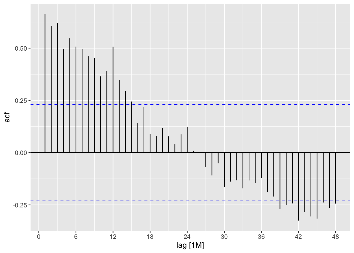
## 8 Western Australia

pigs <- aus_livestock |>
  filter(year(Month) %in% 1990:1995, State == 'Victoria', Animal == 'Pigs')

pigs |> autoplot()

## Plot variable not specified, automatically selected `.vars = Count`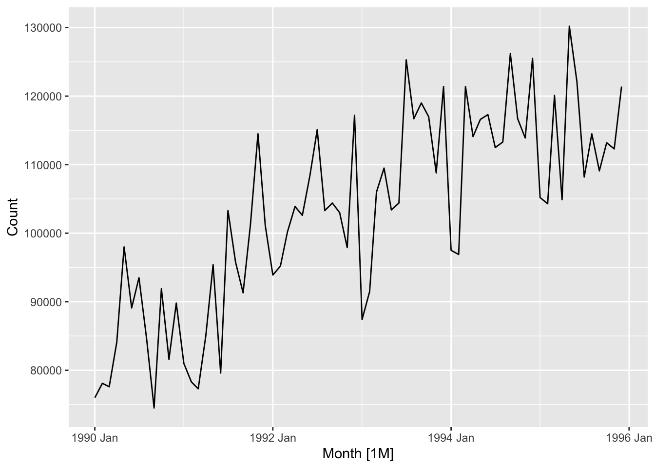

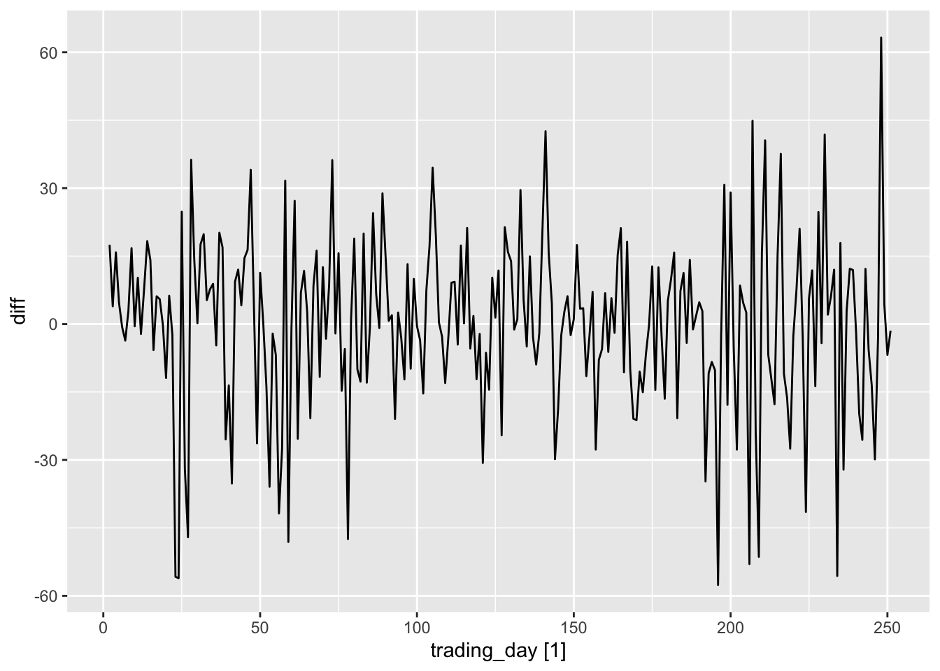
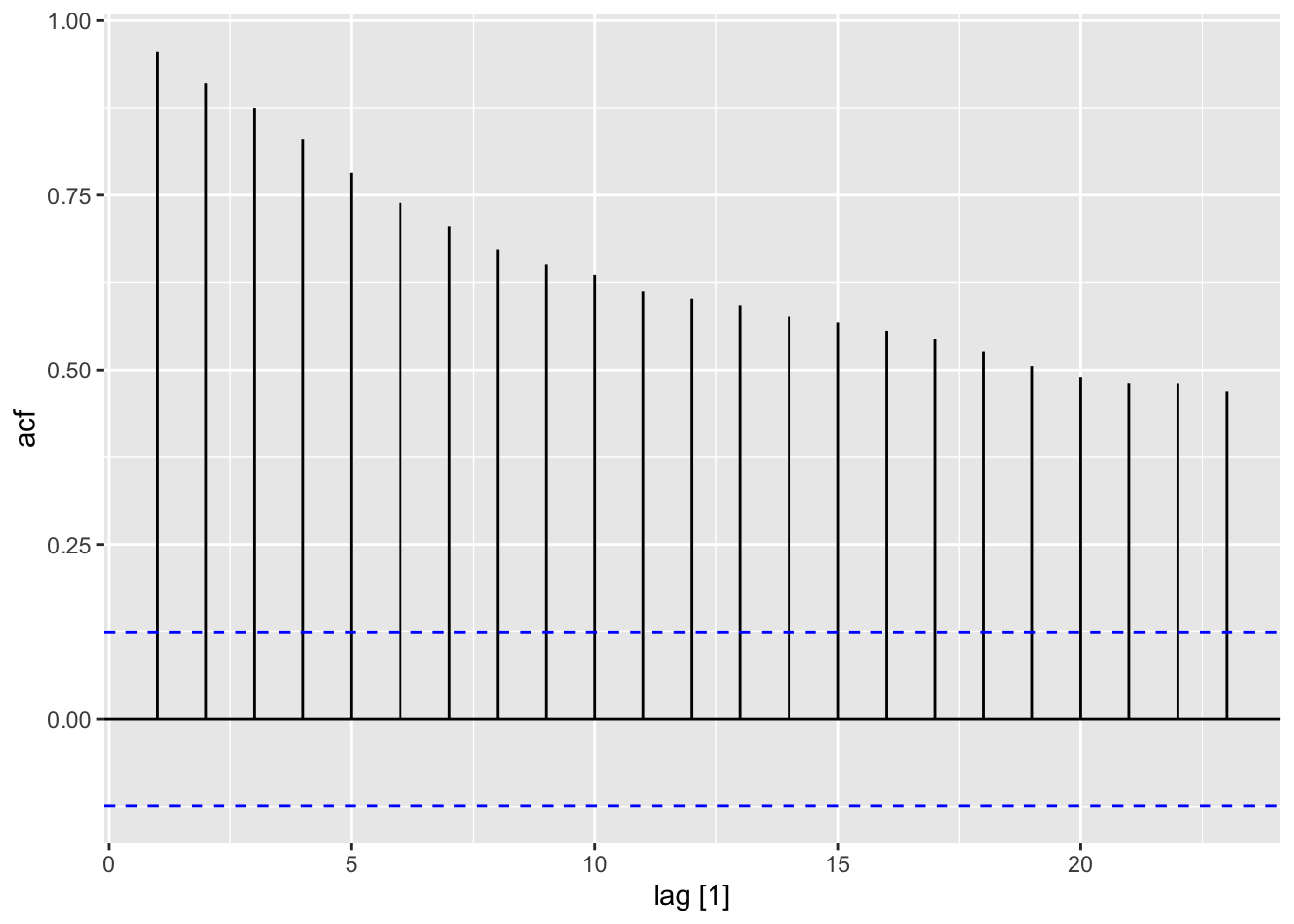
pigs |> ACF(Count, lag_max = 48) |> autoplot()

dgoog <- gafa_stock |>
  filter(Symbol == "GOOG", year(Date) >= 2018) |>
  mutate(trading_day = row_number()) |>
  update_tsibble(index = trading_day, regular = TRUE) |>
  mutate(diff = difference(Close))

dgoog |> autoplot(Close)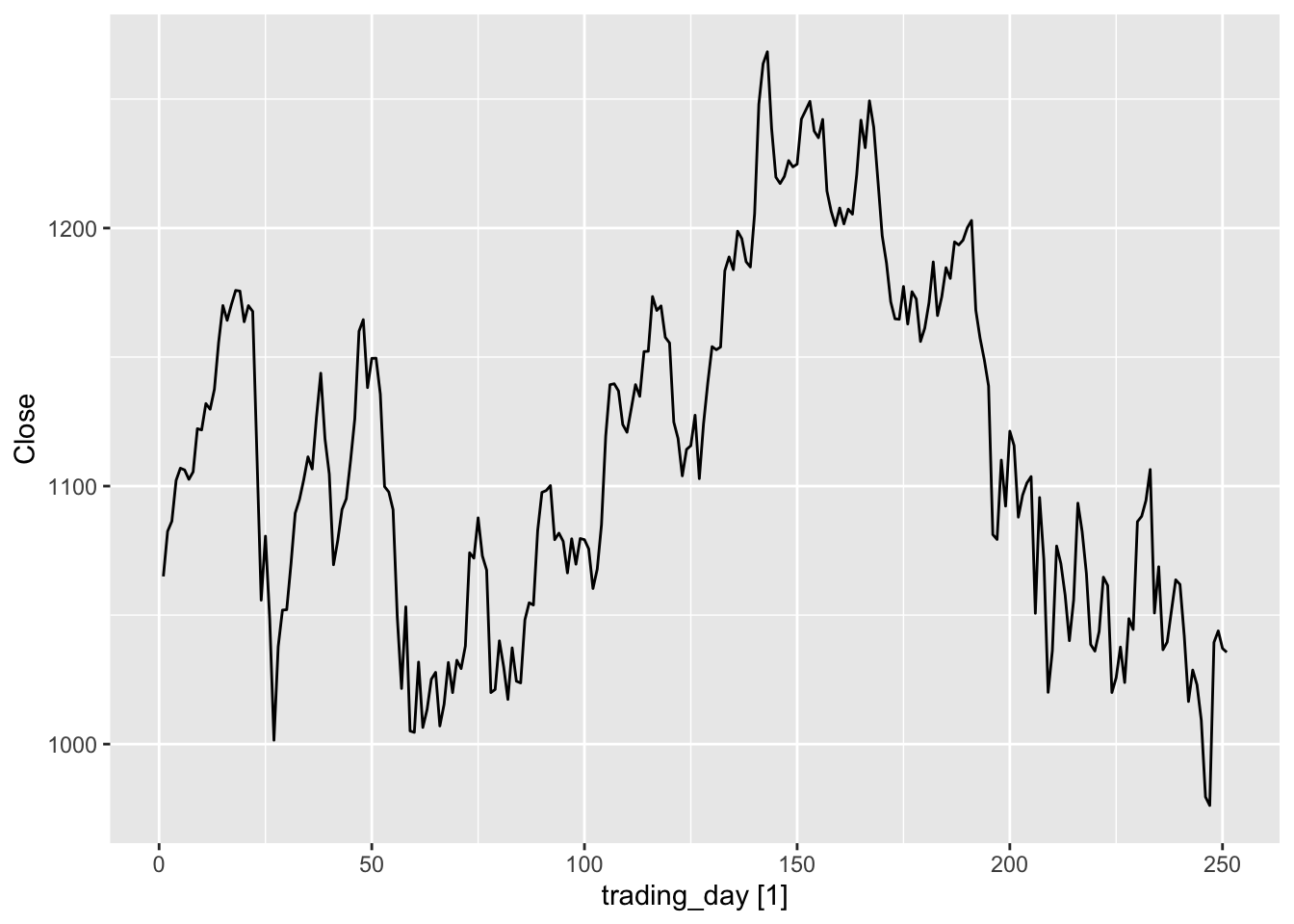

dgoog |> ACF(Close) |> autoplot()

dgoog |> autoplot(diff)

## Warning: Removed 1 row containing missing values or values outside the scale range (`geom_line()`).

dgoog |> ACF(diff) |> autoplot()