Chapter 8 Exponential Smoothing

# loading libraries
library(tsibble)
library(tsibbledata)
library(tidyverse)
# to read data
library(rio)
library(ggplot2)
library(fabletools)
library(feasts)
library(fpp3)
library(latex2exp)
library(forecast)
library(fma)

The source of the chapter

8.1 Simple exponential smoothing

The source of the section

The SES method is suitable for forecasting data with no clear trend or seasonal pattern.

algeria_economy <- global_economy |>
  filter(Country == 'Algeria')

algeria_economy |>
  autoplot(Exports) +
  labs(y = '% of GDP', title = 'Exports: Algeria')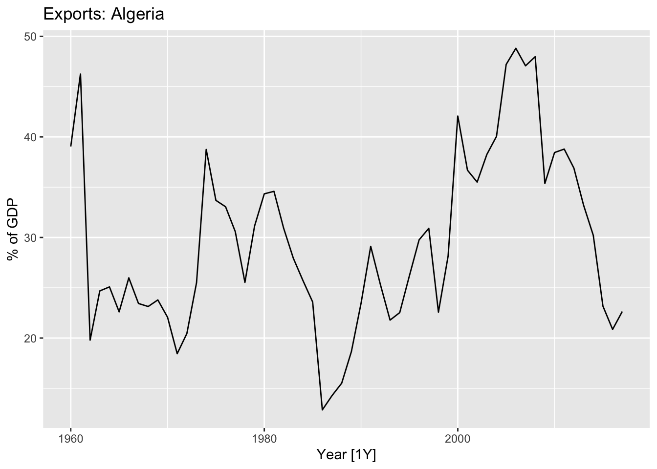

Forecasts are calculated using weighted averages, where the weights decrease exponentially as observations come from further in the past — the smallest weights are associated with the oldest observations.

\[ \hat y_{T+1|T} = \alpha y_T + \alpha(1 - \alpha)y_{T-1} +\alpha(1 - \alpha)^2y_{T-1}+... \]

where \(0 \le \alpha \le 1\) is the smoothing parameter.

8.1.1 Weighted average form

\[ \hat y_{T+1|T} = \alpha y_T + (1-\alpha) \hat y_{T|T-1} \] where \(0 \le \alpha \le 1\) is the smoothing parameter.

\[ \hat y_{T+1|T} = \sum_{j=0}^{T-1} \alpha(1-\alpha)^j y_{T-j} + (a-\alpha)^T\ell_0 \]

The weighted average form leads to the same forecast equation of simple exponential smoothing.

8.1.2 Component form

Forecast:

\[ \hat y_{t+h|t} = \ell_t \] Smoothing:

\[ \ell_t = \alpha y_t + (1- \alpha)\ell_{t-1} \]

8.1.3 Flat forecast

\[ \hat y_{T+h|T} = \hat y_{T+1|T} = \ell_T, \space \space \space h = 2,3,... \] > That is, all forecasts take the same value, equal to the last level component. Remember that these forecasts will only be suitable if the time series has no trend or seasonal component.

8.1.4 Optimisation

The unknown parameters (\(\alpha\)) and the initial values (\(\ell_0\)) for any exponential smoothing method can be estimated by minimising the SSE.

\[ SSE = \sum_{t=1}^T(y_t - \hat y_{t|t-1})^2 = \sum_{t=1}^T e_t^2 \]

where \(e_t = y_t - \hat y_{t|t-1}\) for \(t=1,...,T\)

8.1.5 Example: Algerian exports

Fit the model ETS(ANN).

# Estimate parameters
fit <- algeria_economy |>
  model(ETS(Exports ~ error("A") + trend("N") + season("N")))
fc <- fit |>
  forecast(h = 5)

Model report.

fit |> report()

## Series: Exports 
## Model: ETS(A,N,N) 
##   Smoothing parameters:
##     alpha = 0.8399875 
## 
##   Initial states:
##    l[0]
##  39.539
## 
##   sigma^2:  35.6301
## 
##      AIC     AICc      BIC 
## 446.7154 447.1599 452.8968

The 5-step forecast.

fc

## # A fable: 5 x 5 [1Y]
## # Key:     Country, .model [1]
##   Country .model                                                        Year    Exports .mean
##   <fct>   <chr>                                                        <dbl>     <dist> <dbl>
## 1 Algeria "ETS(Exports ~ error(\"A\") + trend(\"N\") + season(\"N\"))"  2018  N(22, 36)  22.4
## 2 Algeria "ETS(Exports ~ error(\"A\") + trend(\"N\") + season(\"N\"))"  2019  N(22, 61)  22.4
## 3 Algeria "ETS(Exports ~ error(\"A\") + trend(\"N\") + season(\"N\"))"  2020  N(22, 86)  22.4
## 4 Algeria "ETS(Exports ~ error(\"A\") + trend(\"N\") + season(\"N\"))"  2021 N(22, 111)  22.4
## 5 Algeria "ETS(Exports ~ error(\"A\") + trend(\"N\") + season(\"N\"))"  2022 N(22, 136)  22.4

fc |>
  autoplot(algeria_economy) +
  autolayer(fit |> augment(), .fitted, color = 'blue') +
  labs(y="% of GDP", title="Exports: Algeria") +
  guides(colour = "none")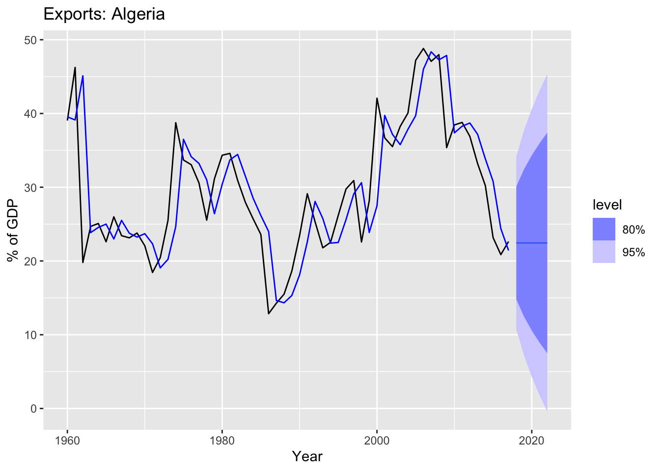

8.2 Methods with trend

The source of the section

8.2.1 Holt’s linear trend method

Forecast: \[ \hat y_{t+h|t} = \ell_t + hb_t \]

Level: \[ \ell_t = \alpha y_t + (1-\alpha)(\ell_{t-1} + b_{t-1}) \]

Trend: \[ b_t = \beta(\ell_t - \ell_{t-1}) + (1-\beta)b_{t-1} \]

Parameters:

• \(\ell_t\) - the level fot he time series at time \(t\)
• \(b_t\) trend (slope) of the time series at time \(t\)
• \(\alpha\) - the smoothing parameter for the level \(0 \le \alpha \le 1\)
• \(\beta\) smoothing parameter for the trend \(0 \le \beta \le 1\)

8.2.1.1 Example: Australian population

aus_economy <- global_economy |>
  filter(Code == "AUS") |>
  mutate(Pop = Population / 1e6)
autoplot(aus_economy, Pop) +
  labs(y = "Millions", title = "Australian population")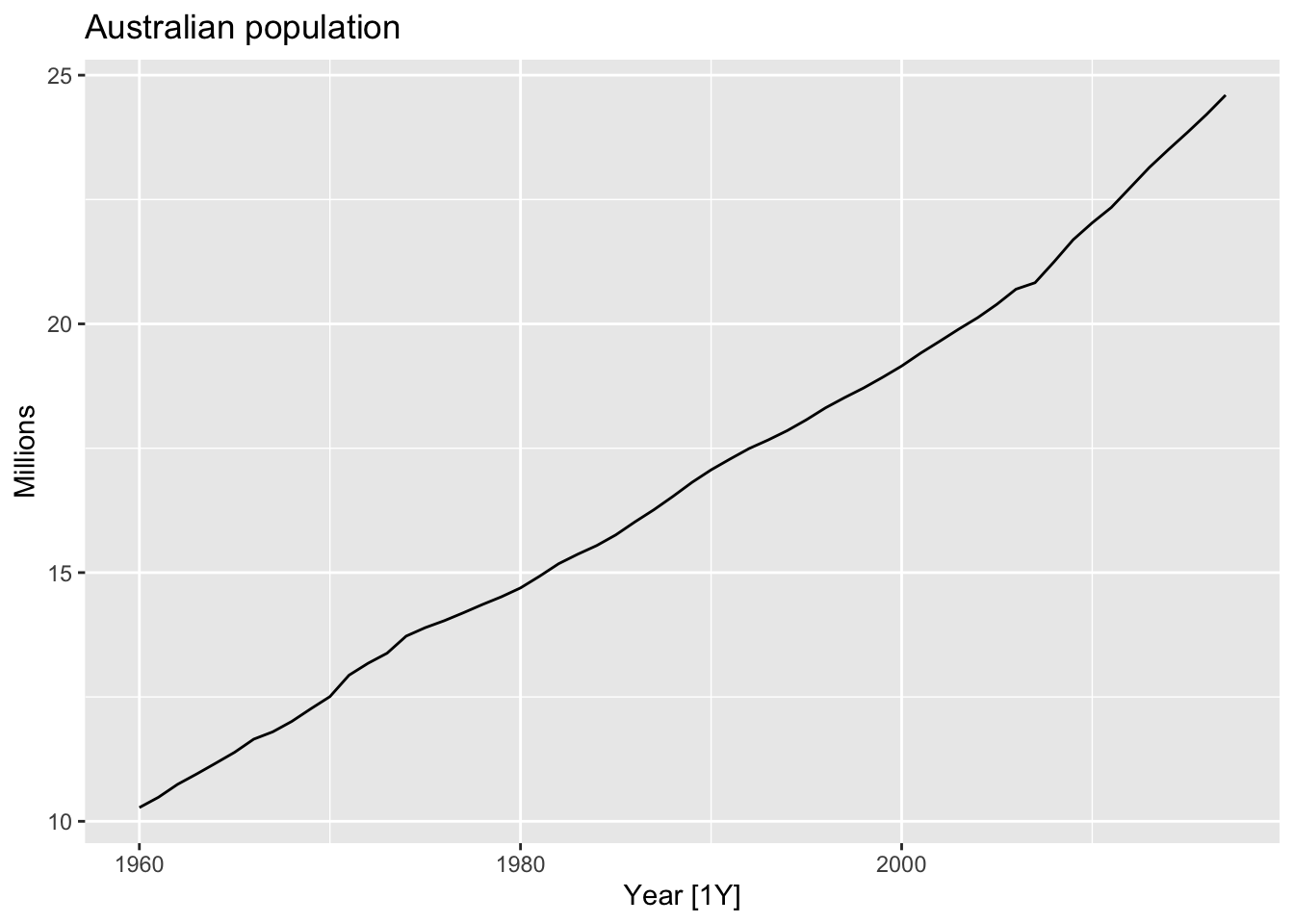

aus_economy |>
  gg_tsdisplay()

## Plot variable not specified, automatically selected `y = GDP`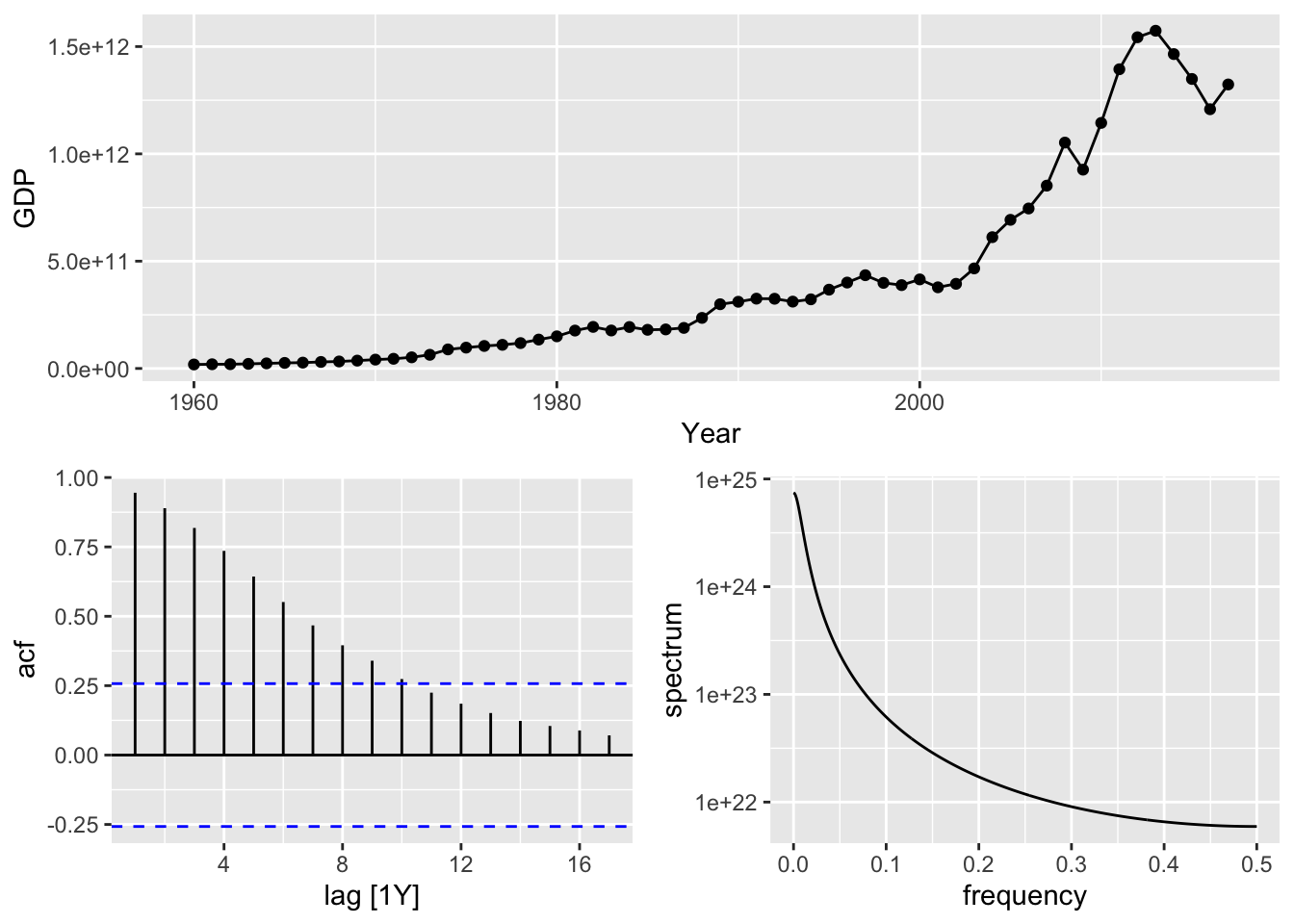

There are trend and no seasonality in the time series, so use ETS(AAN) - Additive error, Additive trend and Non-seasonality.

Fit the model and forecast.

The smoothing parameters, \(\alpha\) and \(\beta\), and the initial values \(\ell_0\) and \(b_0\) are estimated by minimising the SSE for the one-step training errors.

# ETS(AAN) - Additive error, Additive trend and non-seasonality
aus_economy |>
  model(AAN = ETS(Pop ~ error('A') + trend('A') + season('N'))) |>
  forecast(h = 10) |>
  autoplot(aus_economy) +
    labs(y = "Millions", title = "Australian population forecast ETS(AAN)")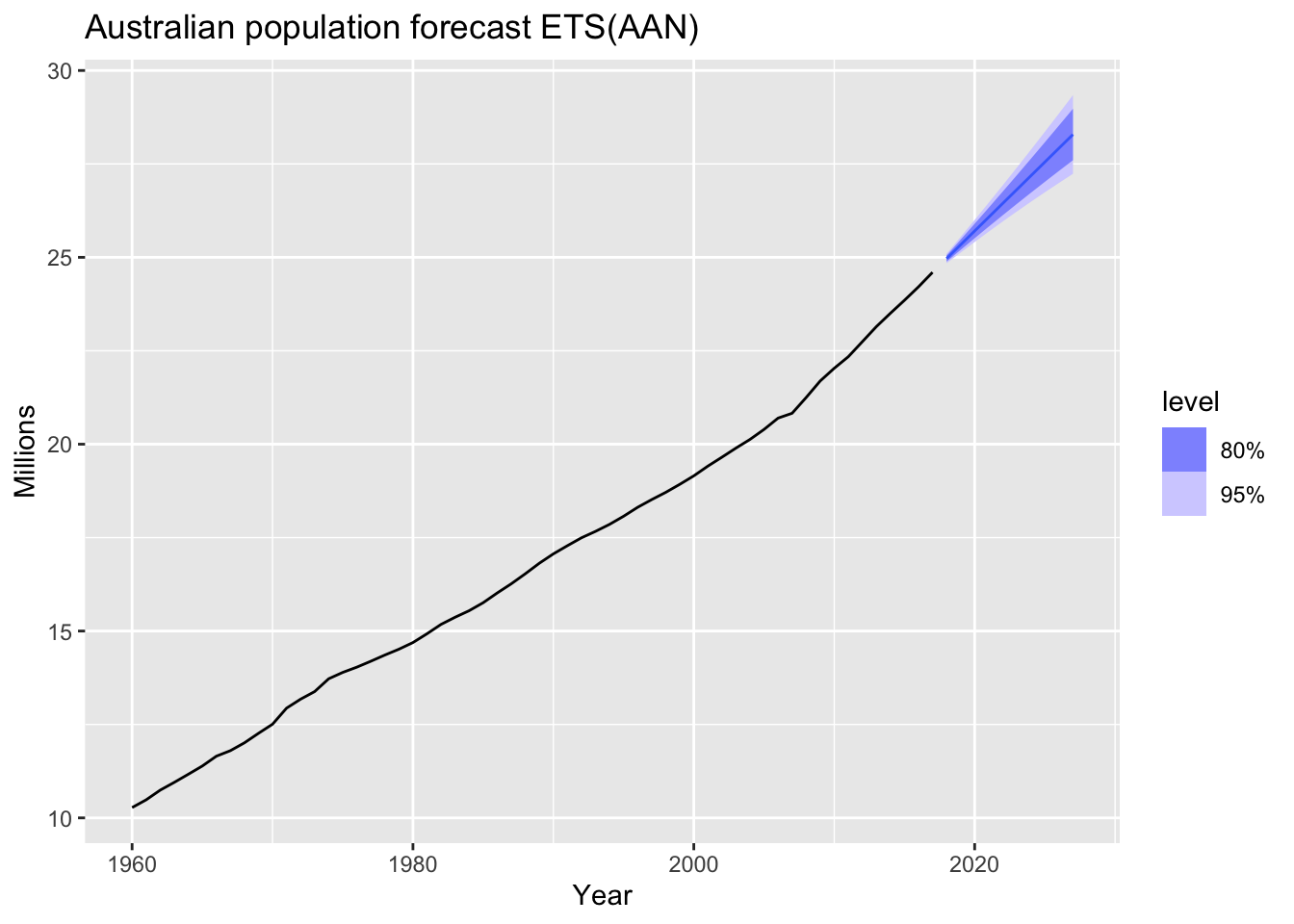

Note! The forecasts generated by EST(AAN) display a constant trend (increasing or decreasing) indefinitely into the future.

8.2.2 Damped trend methods

Forecast: \[ \hat y_{t+h|t} = \ell_t + \left( \sum_{t=1}^h {\phi}^h \right) \times hb_t \]

Level: \[ \ell_t = \alpha y_t + (1-\alpha)(\ell_{t-1} + \phi b_{t-1}) \]

Trend: \[ b_t = \beta(\ell_t - \ell_{t-1}) + (1-\beta)\phi b_{t-1} \]

Parameters:

• \(\ell_t\) - the level fot he time series at time \(t\)
• \(b_t\) trend (slope) of the time series at time \(t\)
• \(\alpha\) - the smoothing parameter for the level \(0 \le \alpha \le 1\)
• \(\beta\) smoothing parameter for the trend \(0 \le \beta \le 1\)
• \(\phi\) a damping parameters \(0 \le \phi \le 1\)

In practice, \(\phi\) is rarely less than 0.8 as the damping has a very strong effect for smaller values. Values of \(\phi\) close to 1 will mean that a damped model is not able to be distinguished from a non-damped model. For these reasons, we usually restrict \(\phi\) to a minimum of 0.8 and a maximum of 0.98.

8.2.2.1 Example: Australian population

There are increasing trend and no seasonality in the aus_economy time series, so use ETS(AAdN) - Additive error, Additive damped trend and Non-seasonality.

Fit the model and forecast.

# ETS(AAdN) - Additive error, Additive damped trend and non-seasonality
aus_economy |>
  model(AAN = ETS(Pop ~ error('A') + trend('A') + season('N')),
        AAdN = ETS(Pop ~ error('A') + trend('Ad', phi = 0.9) + season('N'))) |>
  forecast(h = 15) |>
  autoplot(aus_economy, level=NULL) +
    labs(y = "Millions", title = "Australian population forecast ETS(AAdN)")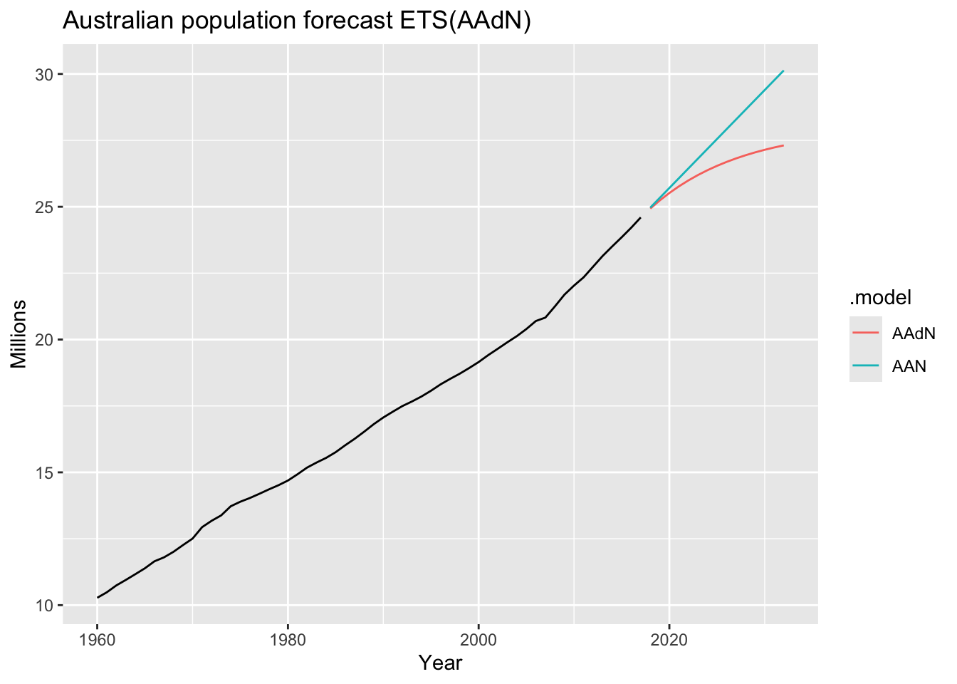

The more \(phi\) is, the mode damping effect.

8.2.2.2 Example: Internet usage

www_usage <- as_tsibble(WWWusage)
www_usage |> autoplot(value) +
  labs(x="Minute", y="Number of users",
       title = "Internet usage per minute")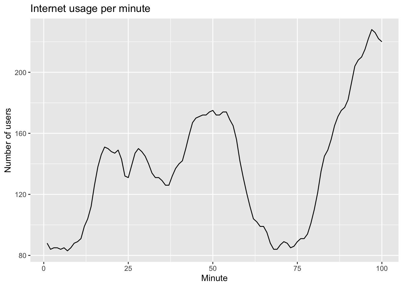

8.2.2.2.1 Cross-validation

www_usage |>
  stretch_tsibble(.init = 10) |>
  model(
    SES = ETS(value ~ error("A") + trend("N") + season("N")),        # ETS(ANN)
    Holt = ETS(value ~ error("A") + trend("A") + season("N")),       # ETS(AAN)
    Damped = ETS(value ~ error("A") + trend("Ad") + season("N"))) |> # ETS(AAdN)
  forecast(h = 1) |>
  accuracy(www_usage) |>
  select(.model, MAE, RMSE, MAPE, MASE)

## Warning: The future dataset is incomplete, incomplete out-of-sample data will be treated as missing. 
## 1 observation is missing at 101

## # A tibble: 3 × 5
##   .model   MAE  RMSE  MAPE  MASE
##   <chr>  <dbl> <dbl> <dbl> <dbl>
## 1 Damped  3.00  3.69  2.26 0.663
## 2 Holt    3.17  3.87  2.38 0.701
## 3 SES     4.81  6.05  3.55 1.06

The damped model ETS(AAdN) is more preferable.

fit <- www_usage |>
  model(
    Damped = ETS(value ~ error("A") + trend("Ad") + season("N"))
  )

fit |> report()

## Series: value 
## Model: ETS(A,Ad,N) 
##   Smoothing parameters:
##     alpha = 0.9999 
##     beta  = 0.9966439 
##     phi   = 0.814958 
## 
##   Initial states:
##      l[0]        b[0]
##  90.35177 -0.01728234
## 
##   sigma^2:  12.2244
## 
##      AIC     AICc      BIC 
## 717.7310 718.6342 733.3620

fit |> tidy()

## # A tibble: 5 × 3
##   .model term  estimate
##   <chr>  <chr>    <dbl>
## 1 Damped alpha   1.00  
## 2 Damped beta    0.997 
## 3 Damped phi     0.815 
## 4 Damped l[0]   90.4   
## 5 Damped b[0]   -0.0173

Make forecasts.

fit |>
  forecast(h = 10) |>
  autoplot(www_usage) +
  labs(x="Minute", y="Number of users",
       title = "Internet usage per minute")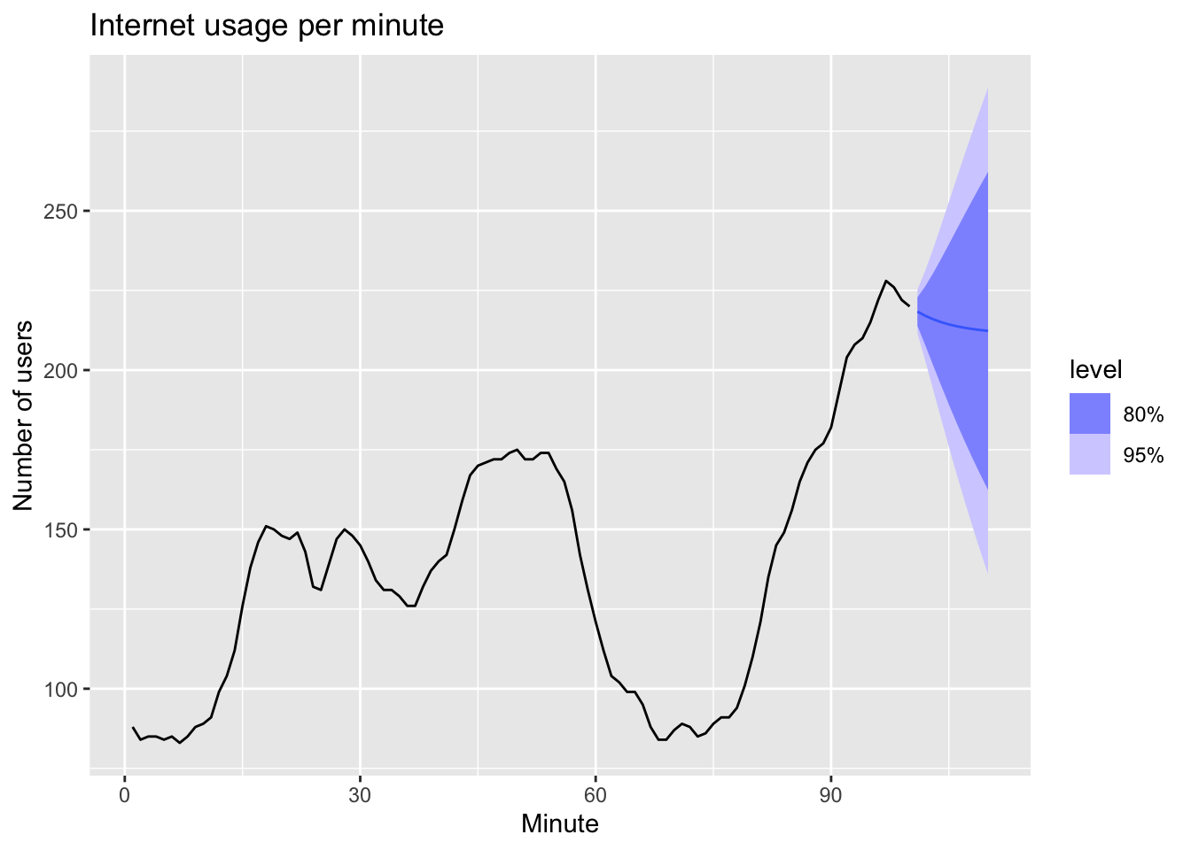

8.3 Methods with seasonality

The source of the section

8.3.1 Holt-Winters’ additive method

Forecast: \[ \hat y_{t+h|t} = \ell_t + hb_t + s_{t + h - m(k-1)} \]

Level: \[ \ell_t = \alpha (y_t - s_{t-m}) + (1-\alpha)(\ell_{t-1} + b_{t-1}) \]

Trend: \[ b_t = \beta(\ell_t - \ell_{t-1}) + (1-\beta)\phi b_{t-1} \]

Season: \[ s_t = \gamma(y_t - \ell_{t-1} - b_{t-1}) + (1-\gamma)s_{t-m} \]

where \(k = (h-1)/m\)

8.3.2 Holt-Winters’ multiplicative method

Forecast:

\[ \hat y_{t+h|t} = (\ell_t + hb_t) \times s_{t + h - m(k+1)} \]

Level:

\[ \ell_t = \alpha \frac {y_t} {s_{t-m}} + (1-\alpha)(\ell_{t-1} + b_{t-1}) \]

Trend:

\[ b_t = \beta(\ell_t - \ell_{t-1}) + (1-\beta) b_{t-1} \]

Season:

\[ s_t = \gamma \frac {y_t} {(\ell_{t-1} + b_{t-1})} + (1-\gamma)s_{t-m} \]

8.3.3 Example: Domestic overnight trips in Australia

aus_holidays <- tourism |>
  filter(Purpose == 'Holiday') |>
  summarise(Trips = sum(Trips)/1e3)

train <- aus_holidays |>
  filter(year(Quarter) < 2015)

#fit the model
fit <- train |>
  model(
    snaive = SNAIVE(Trips), # Seasonal NAIVE
    additive = ETS(Trips ~ error('A') + trend('A') + season('A')), # EST(AAA)
    multiplicative = ETS(Trips ~ error('M') + trend('A') + season('M')) # ETS(MAM)
    )

# make forecats
fc <- fit |> forecast(h = '3 years')

# plot the forecasts
fc |>
  autoplot(aus_holidays, level = NULL) +
  labs(title="Australian domestic tourism",
       y="Overnight trips (millions)") +
  guides(colour = guide_legend(title = "Forecast"))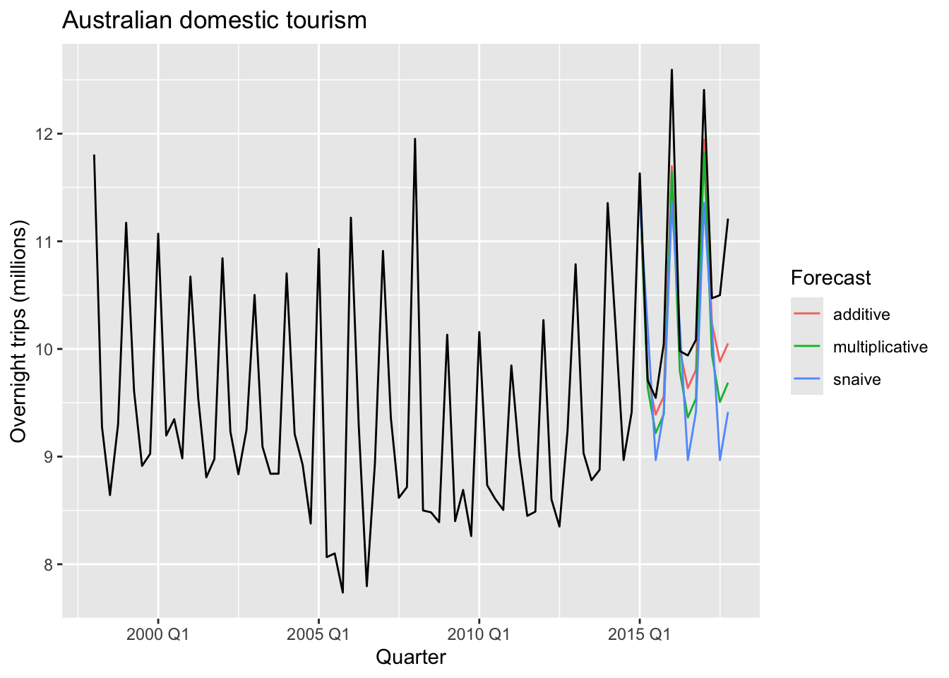

fc |> accuracy(aus_holidays)

## # A tibble: 3 × 10
##   .model         .type    ME  RMSE   MAE   MPE  MAPE  MASE RMSSE   ACF1
##   <chr>          <chr> <dbl> <dbl> <dbl> <dbl> <dbl> <dbl> <dbl>  <dbl>
## 1 additive       Test  0.394 0.521 0.402  3.56  3.63  1.01 0.981 0.129 
## 2 multiplicative Test  0.591 0.710 0.591  5.45  5.45  1.48 1.34  0.312 
## 3 snaive         Test  0.692 0.948 0.811  6.28  7.49  2.03 1.78  0.0518

fit$additive[[1]] |> report()

## Series: Trips 
## Model: ETS(A,A,A) 
##   Smoothing parameters:
##     alpha = 0.2561579 
##     beta  = 0.02543275 
##     gamma = 0.0001002324 
## 
##   Initial states:
##      l[0]        b[0]      s[0]      s[-1]      s[-2]    s[-3]
##  9.875393 -0.01230462 -0.568823 -0.6761713 -0.2620541 1.507048
## 
##   sigma^2:  0.2046
## 
##      AIC     AICc      BIC 
## 188.5096 191.6131 208.4852

fit$multiplicative[[1]] |> report()

## Series: Trips 
## Model: ETS(M,A,M) 
##   Smoothing parameters:
##     alpha = 0.2466059 
##     beta  = 0.01562941 
##     gamma = 0.0001000005 
## 
##   Initial states:
##      l[0]        b[0]      s[0]     s[-1]     s[-2]    s[-3]
##  9.886961 -0.02459763 0.9401183 0.9262804 0.9724422 1.161159
## 
##   sigma^2:  0.0023
## 
##      AIC     AICc      BIC 
## 186.2399 189.3434 206.2155

8.3.4 Holt-Winters’ damped method

Using the Holt-Winters method for daily data, where seasonal period is \(m=7\).

sth_cross_ped <- pedestrian |>
  filter(Date >= '2016-07-01', Sensor == 'Southern Cross Station') |>
  index_by(Date) |>
  summarise(Count = sum(Count)/1000)

sth_cross_ped |>
  filter(Date <= '2016-07-31') |>
  model(
    hw = ETS(Count ~ error('M') + trend('Ad') + season('M'))
  ) |>
  forecast(h = '2 weeks') |>
  autoplot(sth_cross_ped  |> filter(Date <= "2016-08-14")) +
  labs(title = "Daily traffic: Southern Cross",
       y="Pedestrians ('000)")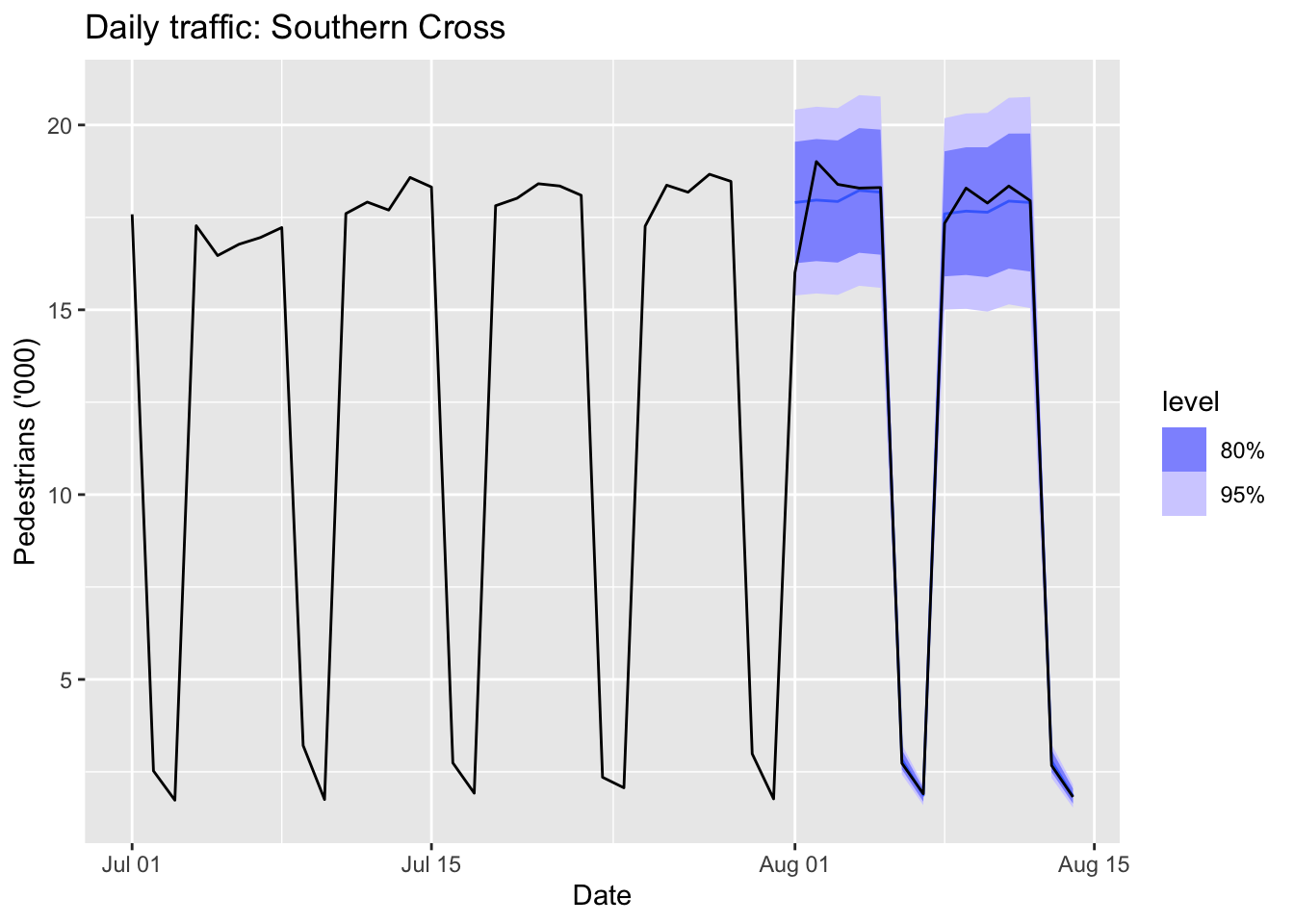

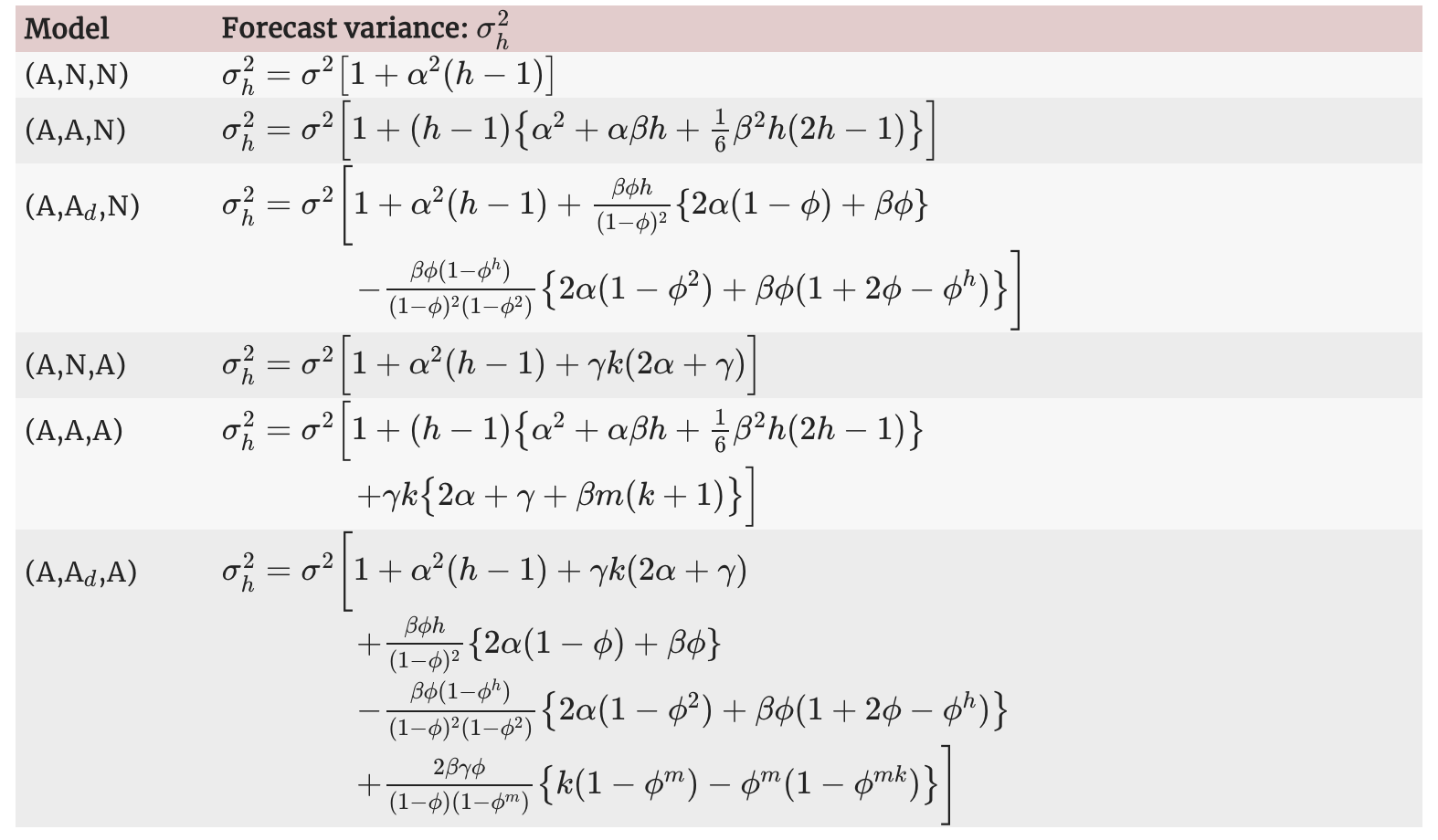
8.4 A taxonomy of exponential smoothing methods

The source of the section

Trend Component	Seasonal Component
	N	A	M
	(None)	(Additive)	(Multiplicative)
N (None)	(N, N)	(N, A)	(N, M)
A (Additive)	(A, N)	(A, A)	(A, M)
\(A_d\) (Additive damped)	(\(A_d\), N)	(\(A_d\), A)	(\(A_d\), M)

Short hand	Method
(N,N)	Simple exponential smoothing
(A,N)	Holt’s linear method
(\(A_d\),N)	Additive damped trend method
(A,A)	Additive Holt-Winters’ method
(A,M)	Multiplicative Holt-Winters’ method
(\(A_d\),M)	Holt-Winters’ damped method

8.5 Innovations state space models for exponential smoothing

The source of the section

ETS : Error, Trend, Seasonal

• Error: {A, M}
• Trend: {N, A, \(A_d\)}
• Seasonal: {N, A, M}

8.6 Estimation and model selection

The source of the section

8.6.1 Model selection

The AIC, \(AIC_c\) and BIC can be used to determine which of the ETS models is most appropriate for a given time series.

Akaike’s Information Criterion (AIC)

\[ AIC = - 2 log(L) + 2k \]

where \(L\) is the likelihood of the model and \(k\) is the total number of parameters and initial states that have been estimated.

The AIC corrected for small sample bias (\(BIC_c\))

\[ AIC_c = AIC + \frac {2k(k+1)}{T-k-1} \] Bayesian Information Criterion (BIC)

\[ BIC = AIC + k[log(T) - 2] \]

8.6.2 Example: Domestic holiday tourist visitor nights in Australia

aus_holidays <- tourism |>
  filter(Purpose == 'Holiday') |>
  summarise(Trips = sum(Trips)/1e3)

fit <- aus_holidays |>
  model(ETS(Trips))

report(fit)

## Series: Trips 
## Model: ETS(M,N,A) 
##   Smoothing parameters:
##     alpha = 0.3484054 
##     gamma = 0.0001000018 
## 
##   Initial states:
##      l[0]       s[0]      s[-1]      s[-2]    s[-3]
##  9.727072 -0.5376106 -0.6884343 -0.2933663 1.519411
## 
##   sigma^2:  0.0022
## 
##      AIC     AICc      BIC 
## 226.2289 227.7845 242.9031

components(fit) |>
  autoplot() +
  labs(title = "ETS(M,N,A) components")

## Warning: Removed 4 rows containing missing values or values outside the scale range (`geom_line()`).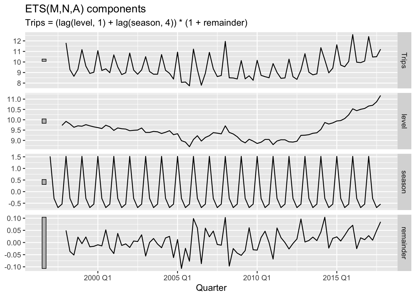

8.7 Forecasting with ETS models

The source of the section

fit |>
  forecast(h = 8) |>
  autoplot(aus_holidays) +
  labs(title="Australian domestic tourism",
       y="Overnight trips (millions)")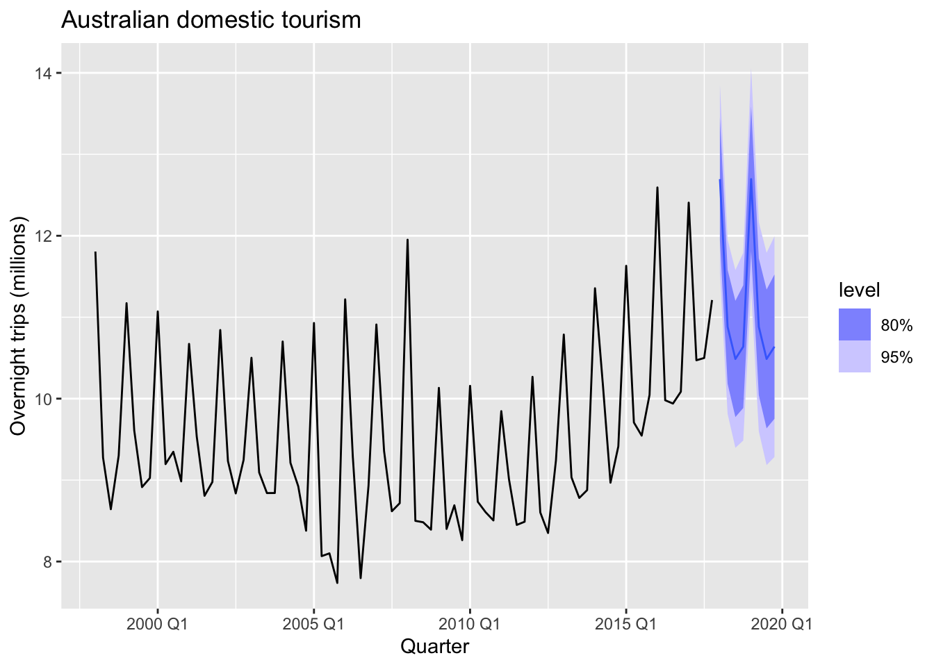

8.7.1 Prediction intervals

\[ \hat y_{T+h|T} \pm c\sigma_h \] where where \(c\) depends on the coverage probability, and \(c\sigma^2_h\) is the forecast variance.

8.8 Excercises

# Simple Exp Smoothing is ETS(ANN)

pigs <- aus_livestock |>
  filter(Animal == 'Pigs', State == 'Victoria')

pigs |>
  autoplot(Count) +
  labs(title = 'Pigs slaughtered in Victoria')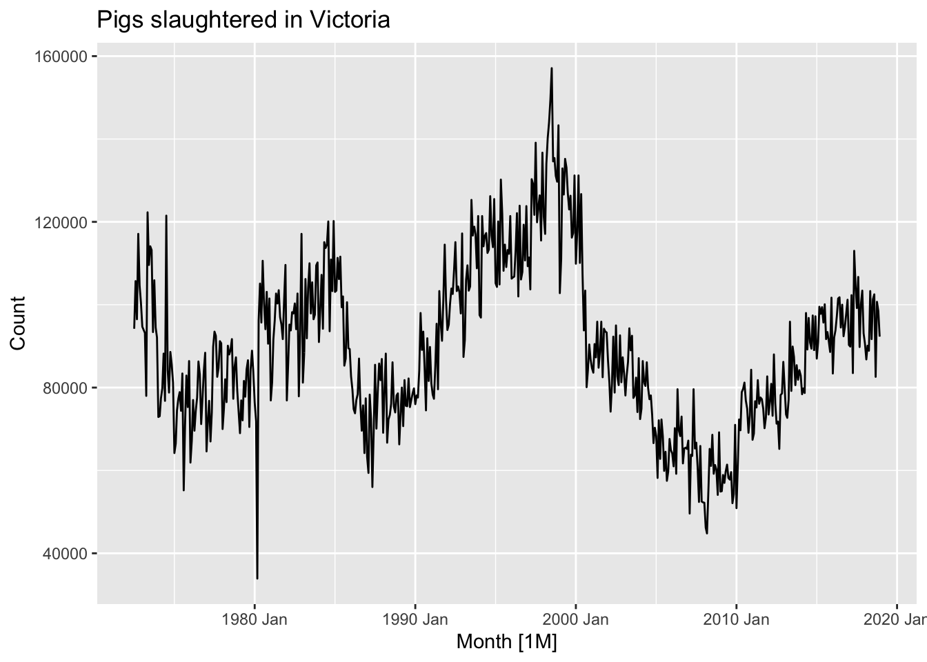

# a. ETS(ANN) - no trend, no seasonality

fit <- pigs |>
  model(ETS(Count ~ error('A') + trend('N') + season('N')))

fit |>
  report()

## Series: Count 
## Model: ETS(A,N,N) 
##   Smoothing parameters:
##     alpha = 0.3221247 
## 
##   Initial states:
##      l[0]
##  100646.6
## 
##   sigma^2:  87480760
## 
##      AIC     AICc      BIC 
## 13737.10 13737.14 13750.07

# forecast
fc <- fit |>
  forecast(h = 4)

fc

## # A fable: 4 x 6 [1M]
## # Key:     Animal, State, .model [1]
##   Animal State    .model                                                        Month             Count  .mean
##   <fct>  <fct>    <chr>                                                         <mth>            <dist>  <dbl>
## 1 Pigs   Victoria "ETS(Count ~ error(\"A\") + trend(\"N\") + season(\"N\"))" 2019 Jan N(95187, 8.7e+07) 95187.
## 2 Pigs   Victoria "ETS(Count ~ error(\"A\") + trend(\"N\") + season(\"N\"))" 2019 Feb N(95187, 9.7e+07) 95187.
## 3 Pigs   Victoria "ETS(Count ~ error(\"A\") + trend(\"N\") + season(\"N\"))" 2019 Mar N(95187, 1.1e+08) 95187.
## 4 Pigs   Victoria "ETS(Count ~ error(\"A\") + trend(\"N\") + season(\"N\"))" 2019 Apr N(95187, 1.1e+08) 95187.

aug <- fit |> augment()

# b
print(paste('PI(1) low: ', round(fc$.mean[1] - 1.96*sd(aug$.resid), 2)))

## [1] "PI(1) low:  76871.01"

print(paste('PI(1) hi: ', round(fc$.mean[1] + 1.96*sd(aug$.resid), 2)))

## [1] "PI(1) hi:  113502.1"

fc |> hilo(level = 95) |>
  filter(month(Month) == 1) |>
  select(`95%`)

## # A tsibble: 1 x 2 [1M]
##                    `95%`    Month
##                   <hilo>    <mth>
## 1 [76854.79, 113518.3]95 2019 Jan

simple_exp_smoothing <- function(y_ts, alpha, level){
  y <- numeric(1) 
  l <- numeric(1)
  f <- numeric(1)
  
  y[1] <- NA
  l[1] <- level
  f[1] <- NA
  
  for (i in 1:(length(y_ts)+1)) {
    y[i+1] <- y_ts[i]
    l[i+1] <- alpha * y[i+1]+(1-alpha)*l[i]
    f[i+1] <- l[i]
  }
  return(f[length(f)])
}

a <- 0.3221247
l0 <- 100646.6

print(paste('SES manual one-step forecast: ', simple_exp_smoothing(pigs$Count, a, l0)))

## [1] "SES manual one-step forecast:  95186.5574351184"

# ETS()
print(paste('ETS(ANN) one-step forecast: ', fc$.mean[1]))

## [1] "ETS(ANN) one-step forecast:  95186.5574309915"

simple_exp_smoothing <- function(y_ts, params){
  y <- numeric(1) 
  l <- numeric(1)
  f <- numeric(1)
  e <- numeric(1)
  
  alpha <- params[1]
  level <- params[2]
  y[1] <- NA
  l[1] <- level
  f[1] <- NA
  e[1] <- NA
  
  for (i in 1:(length(y_ts))) {
    y[i+1] <- y_ts[i]
    l[i+1] <- alpha * y[i+1]+(1-alpha)*l[i]
    f[i+1] <- l[i]
    e[i+1] <- y[i+1] - f[i+1]
  }
  sse <- sum(e^2, na.rm = T)
  return(sse)
}


result <- optim(par=c(alpha = 0, level=0), fn = simple_exp_smoothing, y_ts = pigs$Count, method = "L-BFGS-B", lower = c(0, min(pigs$Count)), upper = c(1, max(pigs$Count)))

print(paste0('Optimal alpha: ', result$par[1]))

## [1] "Optimal alpha: 0.321994872263985"

print(paste0('Optimal level: ', result$par[2]))

## [1] "Optimal level: 100533.064675812"

print(paste0('SSE: ', result$value))

## [1] "SSE: 48639277164.8261"

coef(fit$`ETS(Count ~ error("A") + trend("N") + season("N"))`[[1]])

## # A tibble: 2 × 2
##   term    estimate
##   <chr>      <dbl>
## 1 alpha      0.322
## 2 l[0]  100647.

# Simple Exponential Smoothing
simple_exp_smoothing <- function(data, alpha, level, h = 0){
  y <- numeric(1) 
  l <- numeric(1)
  f <- numeric(1)
  
  y[1] <- NA
  l[1] <- level
  f[1] <- NA
  
  for (i in 1:(length(data) + h)) {
    y[i+1] <- data[i]
    l[i+1] <- alpha * y[i+1]+(1-alpha)*l[i]
    f[i+1] <- l[i]
  }
  if(h == 0)
    return(f[2:length(f)])
  
  return(f[length(f)])
}

# Sum of squared errors
sse <- function(data, params){
  e <- numeric(1)
  
  alpha <- params[1]
  level <- params[2]
  e[1] <- NA
  f <- simple_exp_smoothing(data, alpha, level)
  sse <- sum((data - f)^2, na.rm = T)
  return(sse)
}

# Find optimal params
optimal_params <- function(data){
  result <- optim(par=c(alpha = 0, level=0), 
                  fn = sse, 
                  data = data, 
                  method = "L-BFGS-B", 
                  lower = c(0, min(data)), 
                  upper = c(1, max(data)))
  return(result)
}

# SES Forecast
SES_onestep_forecast <- function(data){
  result <- optimal_params(data)
  alpha = result$par[1]
  level = result$par[2]
  
  fc <- simple_exp_smoothing(data, alpha, level, h=1)
  
  return(list(alpha = alpha,
           level = level,
           sse = result$value,
           `one-step forecast` = fc
           ))
}

# Test

SES_onestep_forecast(pigs$Count)

## $alpha
##     alpha 
## 0.3219949 
## 
## $level
##    level 
## 100533.1 
## 
## $sse
## [1] 48639277165
## 
## $`one-step forecast`
## [1] 95186.74

# Data Viz

# a.

nl <- global_economy |>
  filter(Country == 'Netherlands')

nl |>
  autoplot(Exports) +
  labs(title='The Netherlands exports', y = '% of GDP')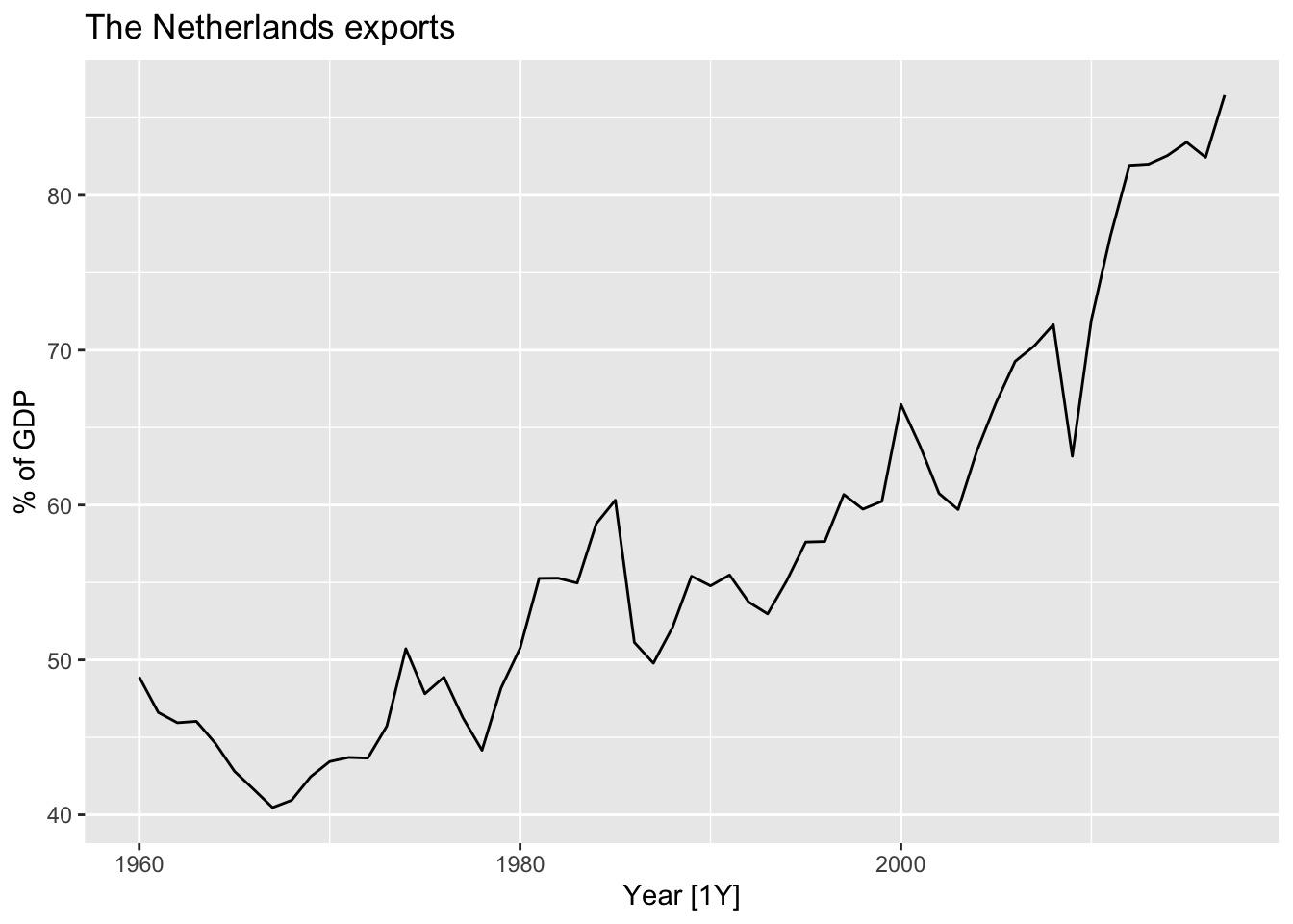

# => Increasing trend and no seasonality (such as it is annual data)

# b. ETS(ANN)

nl |>
  model(ETS(Exports ~ error('A') + trend('N') + season('N'))) |>
  forecast() |>
  autoplot(nl |> filter(Year > 2010))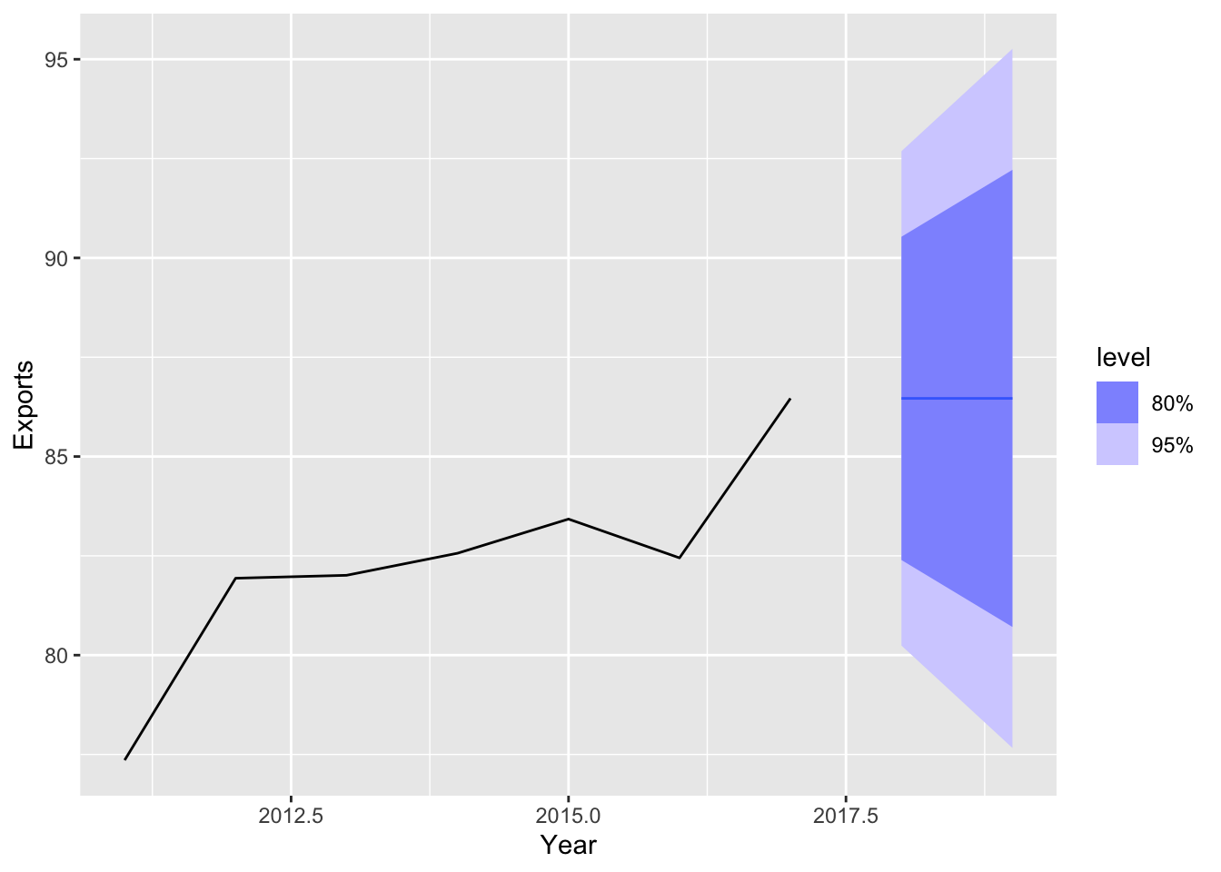

# c

nl |>
  model(ETS(Exports ~ error('A') + trend('N') + season('N'))) |>
  forecast(nl) |>
  accuracy(nl) |>
  select(RMSE)

## # A tibble: 1 × 1
##    RMSE
##   <dbl>
## 1  31.7

# d. ETS(ANN)

nl |>
  model(
    ANN = ETS(Exports ~ error('A') + trend('N') + season('N')),
    AAN = ETS(Exports ~ error('A') + trend('A') + season('N'))) |>
  forecast() |>
  autoplot(nl |> filter(Year > 2010), level = NULL)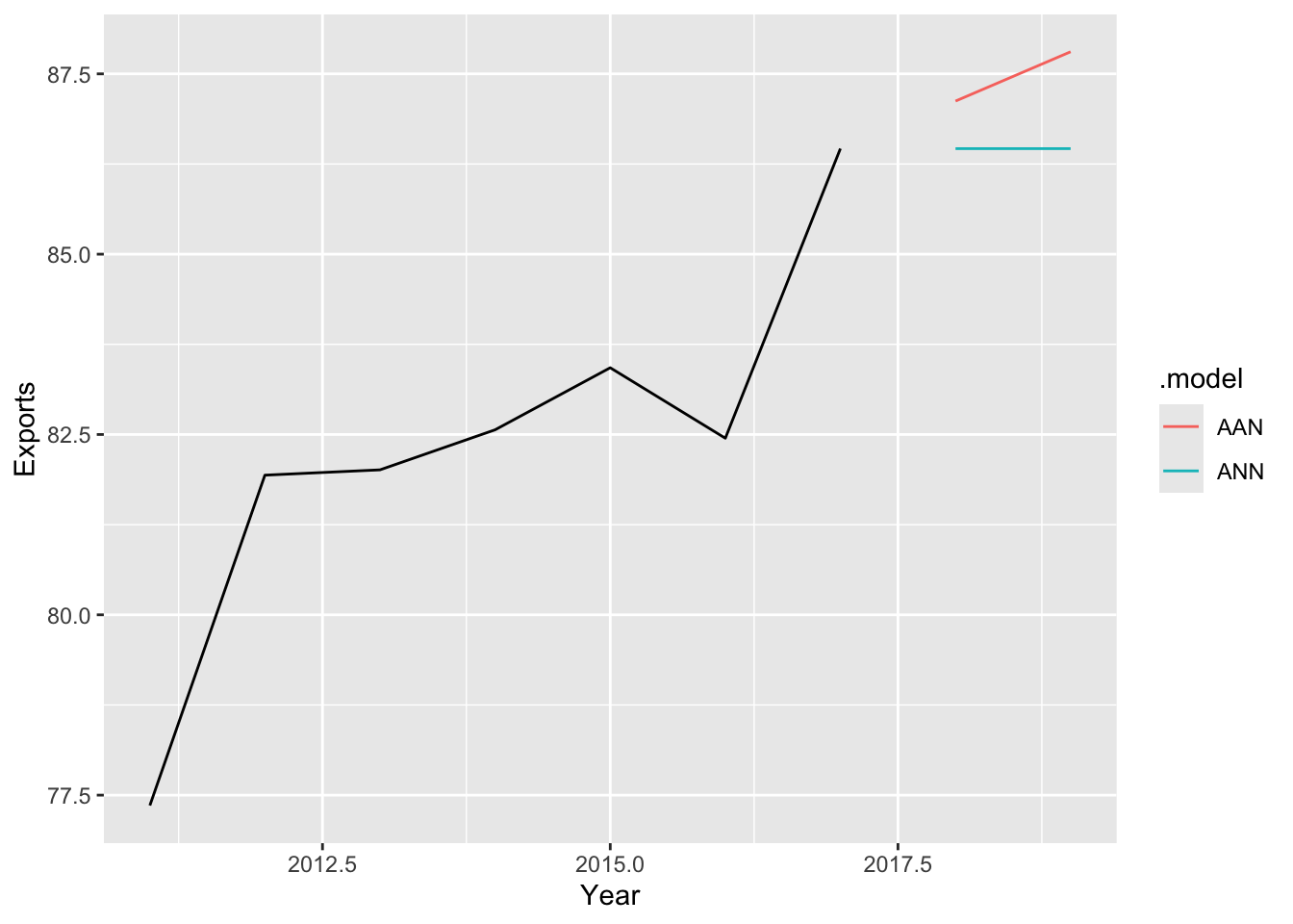

nl |>
  model(
    ANN = ETS(Exports ~ error('A') + trend('N') + season('N')),
    AAN = ETS(Exports ~ error('A') + trend('A') + season('N'))) |>
  forecast(nl) |>
  accuracy(nl) |>
  select(.model, RMSE)

## # A tibble: 2 × 2
##   .model  RMSE
##   <chr>  <dbl>
## 1 AAN     49.6
## 2 ANN     31.7

china <- global_economy |>
  filter(Country == 'China') 

china |>
  autoplot(GDP) +
  labs(title = 'Chinese GDP')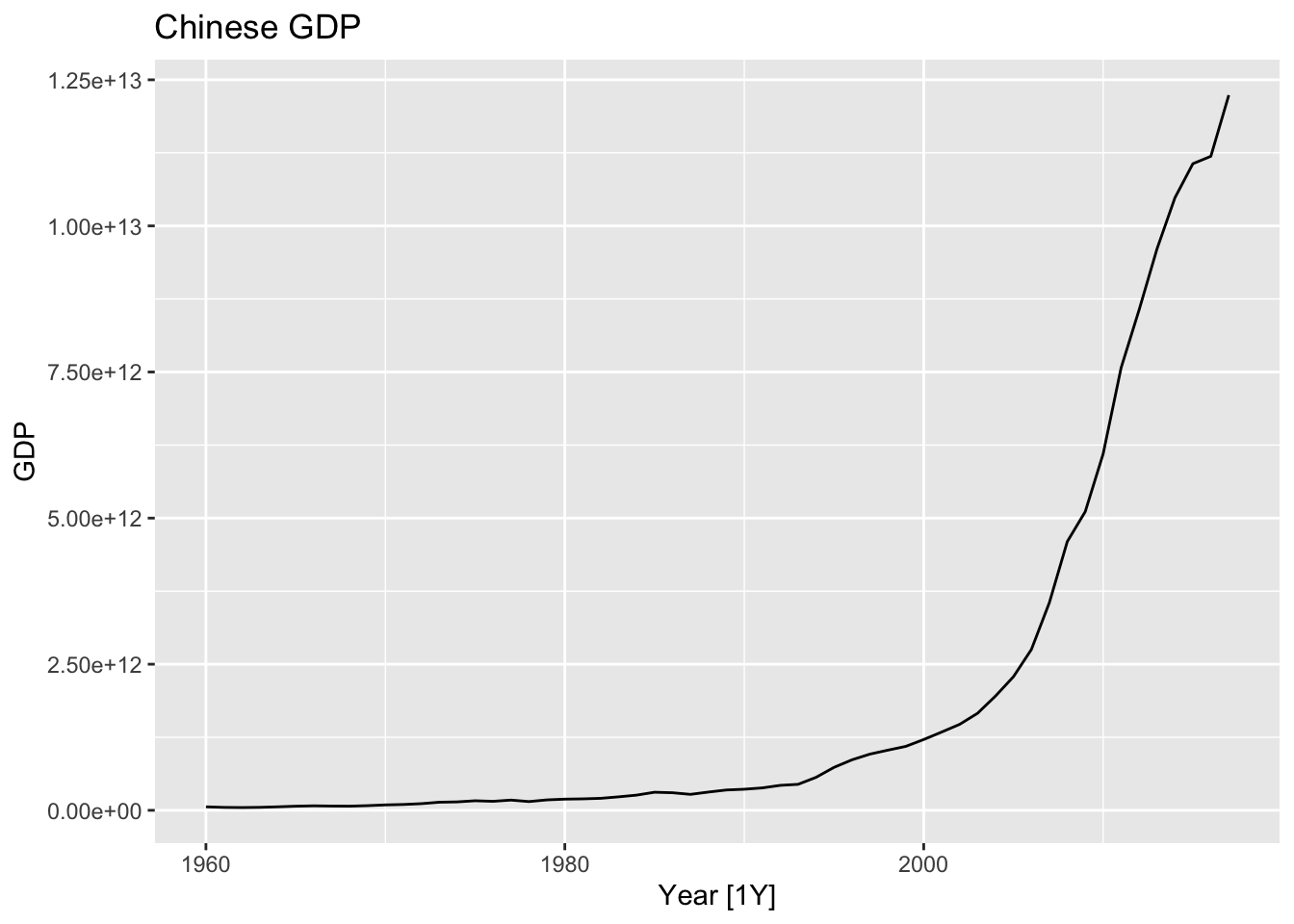

fc <- china |>
  model(
    ANN = ETS(GDP ~ error('A') + trend('N') + season('N')),
    AAN = ETS(GDP ~ error('A') + trend('A') + season('N')),
    AAdN = ETS(GDP ~ error('A') + trend('Ad') + season('N'))
  ) |> 
  forecast(h = '40 years')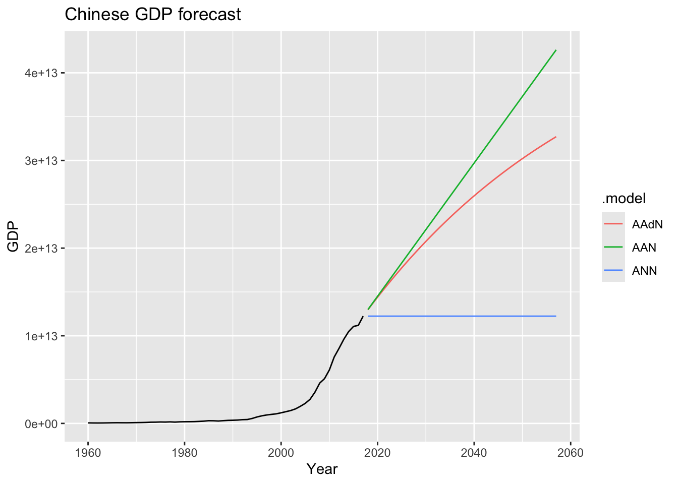

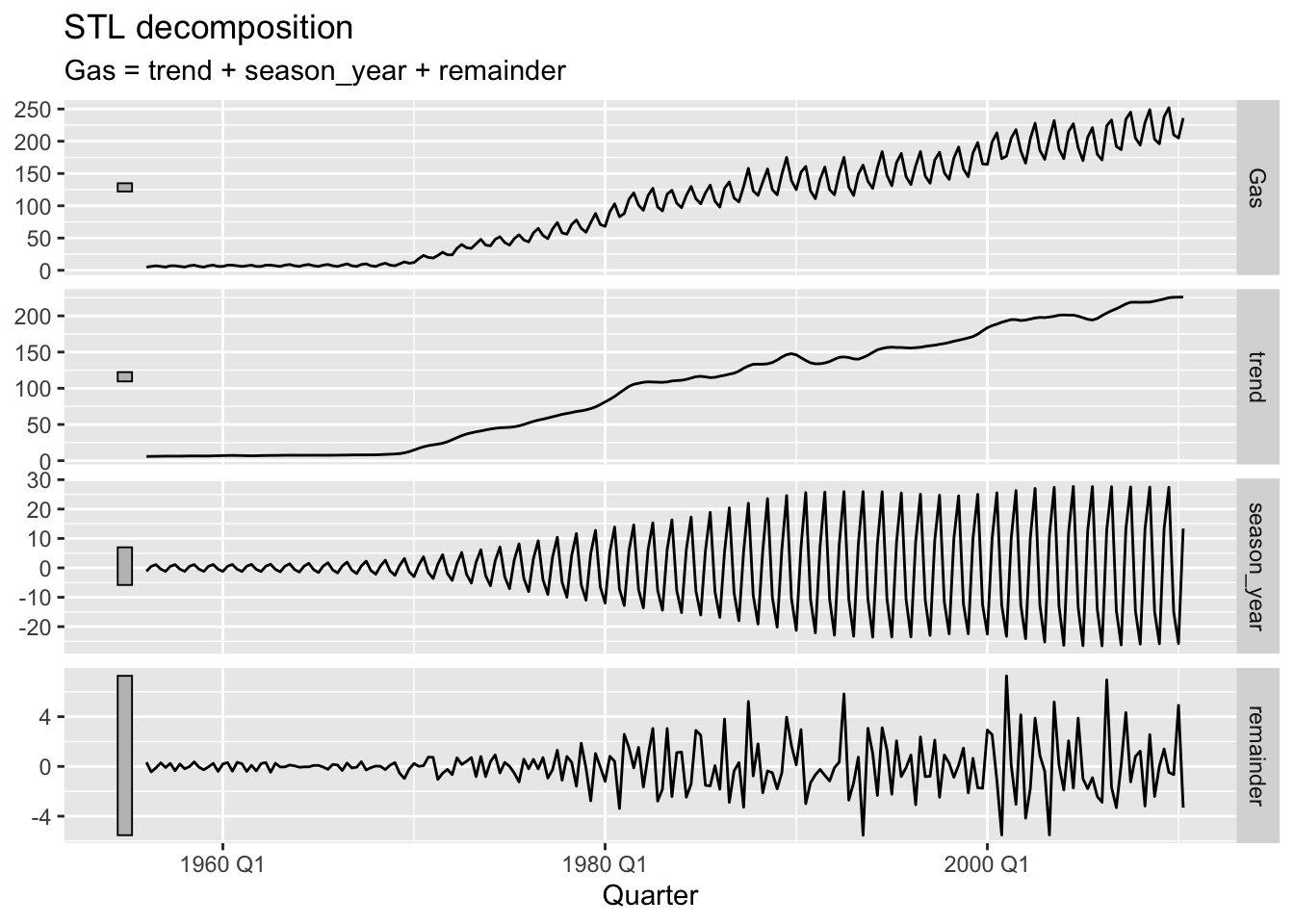
fc |>
  autoplot(china, level = NULL) +
  labs(title = 'Chinese GDP forecast', )

aus_production |>
  model(STL(Gas)) |>
  components() |>
  autoplot()

# unstable seasonal variance and reminder variance => multiplicative seasonality is necessary
fc <- aus_production |>
  model(
    MAM = ETS(Gas ~ error('M') + trend('A') + season('M')),
    MAdM = ETS(Gas ~ error('M') + trend('Ad') + season('M'))
    ) |>
  forecast(h = '5 years') 

fc |>
  autoplot(aus_production |> filter(year(Quarter) > 2005), level = NULL)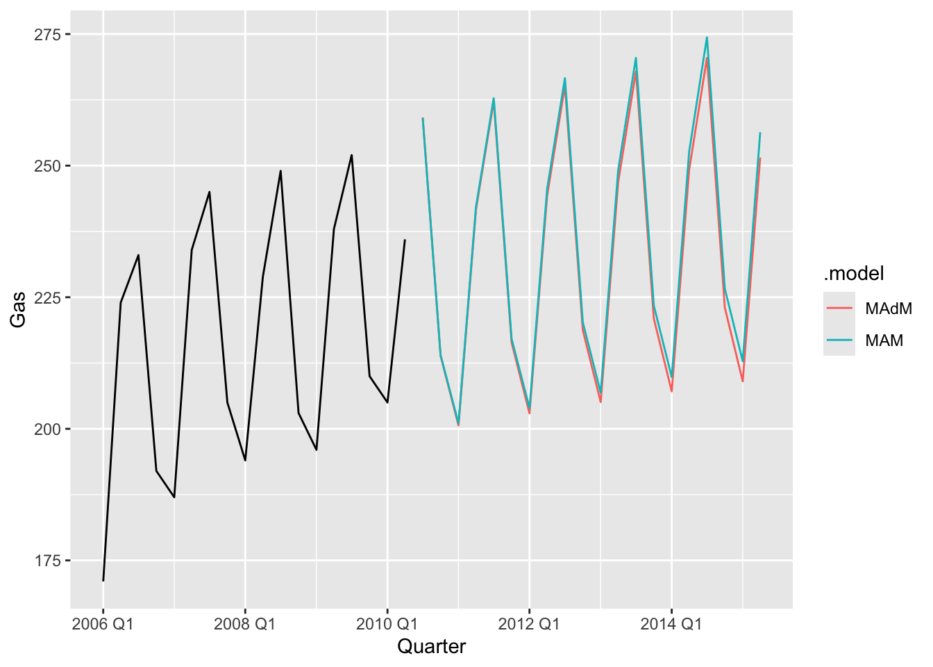

aus_production |>
  model(
    MAM = ETS(Gas ~ error('M') + trend('A') + season('M')),
    MAdM = ETS(Gas ~ error('M') + trend('Ad') + season('M'))
    ) |>
  forecast(aus_production, h = '5 years') |>
  accuracy(aus_production)

## Warning: Input forecast horizon `h` will be ignored as `new_data` has been provided.

## # A tibble: 2 × 10
##   .model .type    ME  RMSE   MAE    MPE  MAPE  MASE RMSSE   ACF1
##   <chr>  <chr> <dbl> <dbl> <dbl>  <dbl> <dbl> <dbl> <dbl>  <dbl>
## 1 MAM    Test  -243.  248.  243. -1116. 1116.   NaN   NaN 0.0567
## 2 MAdM   Test  -167.  181.  167. -1027. 1027.   NaN   NaN 0.678